Archive for January, 2017


FUEL & FUEL SYSTEM MICROBIOLOGY PART 6 – HANDLING SAMPLES

Changes in population as sample ages

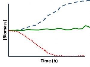
Fig 1. Sample perishability: Changes in population as sample ages


Source: CAERT

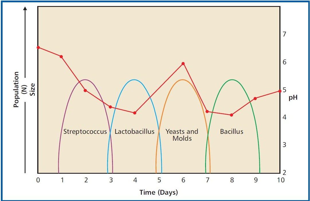
Fig 2. Microbial population succession in Milk. Source: CAERT


Today, I’m returning to the sampling issue that I introduced in Part 2.  In particular, I’ll focus on the concept of sample perishability – the tendency for the contents or properties of a sample to change over time. 

Microbes are living beings.  Like all other living beings, microbes eat, discharge (excrete) wastes, use energy, grow (individual cells get larger), reproduce (proliferate), and respond to their environment.  Samples are perishable because microbes collected in the sample, continue their activities after they have been captured.  They respond to their environment and change it, by using up nutrients and excreting wastes.

Even before active microbes change them, conditions in a sample container are different from those in the system from which the sample was collected.  As a result, microbial populations in sample containers can change in three basic ways:  1) the total number of microbes can change: increasing, decreasing, or remaining approximately the same (in the last case, the number of new cells produces is approximately equal to the number of cells dying); 2) the relative abundance of different types of microbes can change; and 3) the combined (interaction) impacts of these two factors can alter the microbial population in countless ways.

Total bioburden: Figure 1 shows how the total number of cells (bioburden) in a fuel + bottoms-water sample can change as the delay between sampling and testing increases.  Because of these changes, ASTM D7464 recommends that samples be tested within 4h after collections and notes that after 24h, even refrigerated samples are unlikely to have microbial populations that closely resemble those present immediately after the sample was collected.

Relative abundance: Types of microbes that were a major part of the total population in the system from which the sample was collected, are sometimes less able to adapt to the conditions in the sample bottle.  When this happens, both the diversity (number of different types of microbes) and the relative abundance (percentage of the total population each type of microbe represents) can change.  Look at Figure 2. Over the course of the first week or so, after milk is collected, there are typically four major population shifts.  For our purposes the population succession details are unimportant.  What is important is that milk’s microbial population changes dramatically.  The population succession in fuel and fuel-associated water samples has not been well studied, but the evidence that does exist suggests that it does occur. 

Bottom line:  Fuel system samples are perishable because the population beings to change so quickly after samples are collected.  For routine condition monitoring, relative abundance changes aren’t going to affect your action decisions.  However, if the population either increases or decreases dramatically between the time the sample was collected and the time it was tested, operators risk either taking action when it is not needed or failing to take action when it is.  To learn more about fuel system sampling for microbial contamination control, please contact me at fredp@biodeterioration-control.com.

FUEL & FUEL SYSTEM MICROBIOLOGY PART 5 – PREDICTIVE MAINTENANCE (PdM)

I introduced predictive maintenance (PdM) in my last post. Because I didn’t mention preventive maintenance (PM) in that post, I used “PM” as an abbreviation for PdM. After reading Part 4, one of my readers asked me to explain the difference between PM and PdM. I’ll oblige that reader in this post.
The very first collateral duty I was assigned when I reported aboard my first ship, as a fresh-caught Ensign, in January 1971, was to implement the Navy’s new Material Maintenance Management (3-M) System which had arrived onboard days before. The Preventative Maintenance System (PMS) was a major sub-system of 3-M. There it sat in nearly a pallet load of corrugated cardboard boxes; all but one of which was filled with Maintenance Requirement Cards(MRC).
Each MRC provided the details needed to enable a sailor (sometimes more than one sailor) to complete a specific preventive maintenance item. It listed: safety considerations, all materials needed (tools, parts, etc.), estimated time to complete, a step-by-step protocol the qualifications (pay-grade(s)) the sailor(s) needed to have before attempting the maintenance action. The remaining box contained the preventive maintenance scheduling guidance. Each maintenance activity covered by an MRC, was assigned a frequency: daily, weekly, monthly, quarterly, annually, or as required. The Chief Petty Officers and Leading Petty Officers of each division (team of sailors with specific rates – job titles and skill sets) were to develop and maintain weekly, monthly and quarterly charts showing scheduled and completed maintenance. For some reason, I decided to calculate the total number of person hours needed to compete all of the PM requirement. I then computed the total number of person hours available, based on the number of sailors serving on the ship. It turned out that the folks who had developed the 3-M PMS had not done a similar calculation. Had all hands spent 24h/d x 7 d/w x 52 w/y they would have provided just about enough person-hours to complete 40% of the PM labor. Such was my introduction to PM.
Don’t get me wrong, PM was a great innovation for its time. The predetermined maintenance item frequency was based on someone’s best estimate of what needed to be done to minimize the risk of equipment failure. However, it was not data driven. In fact, the 3-M system had a fairly effective feedback component, and before many years passed, the Navy learned that in some cases, maintenance actions actually increased failure risks. I suspect that early PM adapted in industry learned some of the same lessons. Eventually, PdM succeeded PM. In contrast to PM, in which maintenance actions are all given the same priority and are timetable driven, PdM uses trend analysis, condition monitoring (CM) data, asset assessment and cost impact analysis to determent when preventive maintenance actions are needed. The end objective is the same for both PM and PdM, but the latter makes much better use of available resources.
So how do we design fuel system predictive maintenance programs that provide a high return on investment?
Let’s start with cost impact analysis. My experience with microbial audits at fuel retail sites suggests that annual corrective maintenance costs at heavily contaminated sites run $1,500 to $2,500 more than at sites with negligible microbial contamination. I’ve also found that at sites where cars line up to fill-up, 8 gpm dispenser flow rates (instead of 10 gpm) translates into 62,000 fewer gallons sold per dispenser per year. Today, gasoline and diesel are both selling for $2.45/gal. At that price the fuel not sold is worth $152,000. That is opportunity cost. Multiply that number by the number of dispensers on site and the opportunity cost becomes substantial. If the site also has a C-store, estimate the impact of reduced dispenser flow rates on customer satisfaction and C-store traffic/purchases. All you really need to know at the outset is your typical dispenser flow rate, your current fuel price and the number of hours per day during which drivers have to wait in line before pulling up to a dispenser.
In my next What’ New post, I’ll discuss some basic CM tools. In the meantime, if you’d like to learn more, reach out to me at fredp@biodeterioration-control.com.

OUR SERVICES

  • Consulting Services
  • Condition Monitoring
  • Microbial Audits
  • Training and Education
  • Biocide Market Opportunity Analysis
  • Antimicrobial Pesticide Selection

REQUEST INFORMATION


    captcha