Archive for the ‘Detecting Microbes’ Category


COMPARING MICROBIOLOGICAL TEST METHODS – PART 1

The tool you choose depends on the intended use.


Culture Versus Non-Culture Test Methods

History

There is a false impression among microbiologists and non-microbiologists alike that because culture testing has been around since the mid-19th century, it is a reference method (I’m come back to the reference method concept in a bit). The first quantitative culture-based method – the heterotrophic plate count (HPC) first appeared in Standard Methods for the Examination of Water and Wastewater Standard Methods, 11th Edition, 1960. Since then, thousands of variations of the HPC method have been developed. They differ in the nutrients used (1000s of different recipes), growth conditions under which inoculated Petri plates are incubated (100s of temperature, relative humidity, and gas combinations), and how the specimen is introduced to the medium (pour plate, spread plate, and streak plate methods). Because of the variety of plate count protocols, ASTM offers a practice rather than a test method – D5465 Standard Practices for Determining Microbial Colony Counts from Waters Analyzed by Plating Methods.

Alternative Tools for Measuring Microbial Bioburdens

Between 2016 and 2018 I wrote a series of articles in which I explained common types of microbiological test methods (see What’s New from Early and Late December 2016, February, Early and Late July, and August 2017, January and February 2018). As I wrote in 2016, each method contributes to our understanding of microbial contamination. Although each quantifies a different property of microbial bioburden (i.e., the number of microbes present or the concentration of a chemical that is tends to be proportional to the number of microbes present), the data generated by different methods generally agree. As new methods are used, analysts invariably want to know how the results compare against those obtained by culture testing. ASTM E1326 Standard Guide for Evaluating Non-culture Microbiological Tests reviews consideration that should be taken into account when either evaluating the reliability of a new test method or choosing among available methods.

Reference Test Method

A reference test method is one that is known to provide the most accurate and precise indication of the parameter being tested. Accuracy is the degree to which a measurement or test result agrees with the true or accepted value (for example, an atomic clock – accurate to 10−9 seconds per day – is more accurate than a spring-mechanism wristwatch – the best of which are accurate to 1 second per day). Precision is the degree to which repeated measurements agree. Figure 1 illustrates these two concepts. In Figure 1a, the results (dots on the target) are both accurate – clustered around the bullseye – and precise – close together. The dots in Figure 1b are precise, but not accurate – the cluster is distant from the bullseye. The dots in Figure 1c are accurate – they are near the bullseye, but not particularly precise. To assess a method’s accuracy, you must first have a reference standard – a substance with known properties (for time, the internationally recognized reference standard is the second – 9 192 631 770 cycles of radiation corresponding to the transition between two energy levels of the ground state of the cesium-133 atom at 0 °K). There is no reference microbiological test method because:

  • Under a given set of conditions, different microbes will behave differently. Test results will be affected by the types of microbes present.
  • A given microbe will behave differently as test conditions vary.
  • There is no consensus standard, reference microbe.

Fig 1. Accuracy and Precision – a) dots clustered around bullseye illustrate a high degree of accuracy and precision; b) the tight cluster of dots illustrates precise but inaccurate results; c) the wide spread of dots around the bullseye illustrates accurate but imprecise results.

A consensus standard is one that has been developed and approved under the auspices of a standards development organization such as ASTM, AOAC, ISO, and others. Consensus standard test methods include precision statements that cite interlaboratory study-based repeatability and reproducibility variation, and bias.

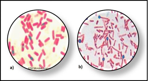
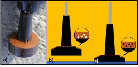
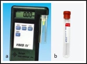
Repeatability is a measure of the variability of results obtained by a single analyst testing replicate specimens from a single sample, using a single apparatus and reagents from single lots. Figure 2 illustrates the repeatability variability for an adenosine triphosphate (ATP) test performed on a metalworking fluid sample. The results are Log10 pg mL-1 where REP is the replicate number and [cATP] is the concentration of cellular ATP per ASTM Test Method E2694.

Fig 2. Repeatability testing – one analyst runs replicate tests on specimens from a single sample, then computes average ( and standard deviation (s). a REP – replicate number; b [cATP] – Log10 pg mL-1.

In comparison, nominal HPC repeatability variation is approximately half an order of magnitude (0.5 Log10 CFU mL-1, where CFU is colony forming units).

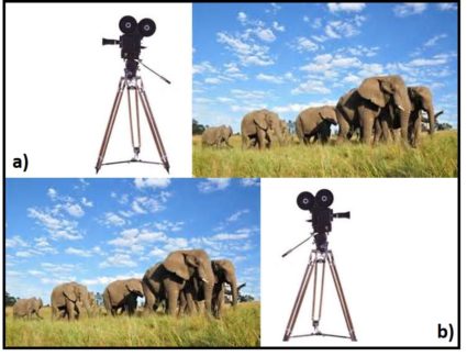
Reproducibility is a measure the variability among multiple analysts running replicate tests on specimens from a single sample, using different sets of apparatus, and reagents. For stable and homogeneous parameters (for example specific gravity) analysts participating in a reproducibility evaluation (interlaboratory study – ILS) are at different facilities. Because microbial contamination is neither homogeneous nor stable, reproducibility testing is commonly performed by analysts at different work-stations located at a single facility. This is called single-site reproducibility testing. Figure 3 illustrates the results of ASTM E2696 reproducibility testing. Ten labs participated in the ILS. The reproducibility standard deviation (sR) was 0.39. Invariably, sR is greater than the repeatability standard deviation (sr).

Fig 3. Reproducibility testing – multiple analysts run the same test on specimens from a sample, using different lab equipment and reagents.

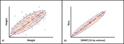
Bias is the difference between a measurement and a parameter’s true value. The cluster of dots in Figure 1b illustrates bias – the distance between the average position of the dots in the cluster and the target’s actual center. Unless there is a reference standard against which a measurement can be compared, only relative bias – the difference between test results obtained by different methods – can be assessed. Figure 4 illustrates bias and relative bias. A water-miscible metalworking fluid (MWF) has been diluted to prepare emulsions with concentrations ([MWF]) of 1, 2, 3, 4 & 5 % v/v. These are the true concentrations ([MWF]T). Each dilution is tested by two methods: refractive index ([MWF]RI) and acid split ([MWF]AS). Each method’s correlation with [MWF]T = 1.0 (0.998 and 0.997 both round to 1.0). However, each has a bias relative to [MWF]T. In this example, [MWF]RI tends to underestimate [MWF] by 16 % and [MWF]AS tends to over-estimate [MWF] by 20 %. The relative bias between the two methods is 36 % – at any [MWF]T, [MWF]AS = 1.20 [MWF]T and 1.36[MWF]RI. Once bias has been determined, it can be used to correct observed values to either true or reference method values.

Fig 4. Bias – graph depicts calibration curves for refractive index (RI) and acid split (AS) metalworking fluid concentration ([MWF]) test methods. [MWF]T is the true (actual) [MWF], [MWF]RI is the concentration as determined by RI, and [MWF]AS is the concentration as determined by AS. The table lists each method’s bias against the [MWF] standards, and the relative bias between the two methods.

As illustrated in figure 5, when two methods measure the same parameter, r is normally expected to be ≈1.0. Bias is only meaningful between two methods used to measure the same parameter (i.e., characteristic or property).

Fig 5. Regression curve – [MWF]RI v. [MWF]AS.

The relationship I’ve used [MWF] test methods to illustrate in this What’s New article is similar to what one would expect when comparing two different culture test methods – for example ASTM D6974 Standard Practice for Enumeration of Viable Bacteria and Fungi in Liquid Fuels—Filtration and Culture Procedures and ASTM D7978 Standard Test Method for Determination of the Viable Aerobic Microbial Content of Fuels and Associated Water—Thixotropic Gel Culture Method. Calibration curves based on dilutions of an original sample with a population density of X (in figure 6, X = 320 CFU mL-1; 2.5Log10 CFU mL-1) are expected to have slopes and r-values ≈1. Because bioburdens can range across ≥5 orders of magnitude (i.e., from <10 CFU mL-1 to >106 CFU mL-1) data are commonly converted from linear to logarithmic (Log10) values. The data in figurer 6 meet our expectations. The trendline’s slope (y) = -0.85 ≈ 1 and r = 1.

Fig 6. Regression curve – Log10 CFU mL-1 v. Log10 dilution factor.

In my next post, I’ll discuss the relationship between methods that measure different but related properties.

Summary

There are a growing number of test methods that can be used to assess bioburdens. Many of these methods quantify the concentration of a biomolecule or class of biomolecules (adenosine triphosphate, carbohydrates, nucleic acids, proteins, etc.). In this article, I reviewed the basic concepts of data variability – repeatability and reproducibility – and bias, and the expected relationship between two methods that purport to measure the same property (for example, two methods to determine [MWF]). In Part 2 I’ll discuss the principles of comparing different methods for assessing microbial bioburden.

As always, I invite your comments and questions. You can reach me at fredp@biodterioration-control.com.

DORMANT MICROBES IN METALWORKING AND OTHER INDUSTRIAL FLUIDS


John Cleese and Michael Palin of Monty Python’s Flying Circus in the “Dead Parrot Sketch”, first aired in December 1969.
What is a dead microbe and why might we care?

I today’s post, I’m returning to a topic I first discussed in 2019 (https://biodeterioration-control.com/2019/07/). In the Monty Python’s Flying Circus “Dead Parrot Sketch”, John Cleese plays the role of an unhappy customer who believes that he has just purchased a dead parrot. Michael Palin – playing the shopkeeper – insists that the parrot is not dead. Rather, it is “simply napping.”

When we monitor microbial contamination in industrial systems, we are typically interested in both how much microbial contamination is present and what damage risk the population poses to the system and the fluids it contains.

Last week, I received an email from a metalworking fluid (MWF) manager who wrote: ““We have another situation with dormant bacteria. In this case we find we have to keep hitting it with biocide more and more often. When the bacteria do start to grow again as the biocide level drops, we see huge pH, alkalinity drops within a week and there is often a bad smell associated. I worry that this is partially due to a large population of dormant bacteria (104 CFU mL-1 to 105 CFU mL-1 on paddles) that is able to wake up and grow more quickly. Is there a way to get at these bacteria and kill them to reduce their population?”

With the MWF manager’s approval, today’s article draws heavily on my response to his email.

Dormant cells

Bacterial endospores

Endospores are special structures formed by a few types of bacteria. Endospores are metabolically inactive (i.e., dormant). There have been reports of microbiologists inducing endospores that have been dormant for more than a million years to germinate into vegetative (i.e., metabolically active) cells. Until recently (i.e., the past ~ 15 years), microbiologists believed that only endospore-forming microbes like Bacillus sp. (Gram +, spore-forming aerobic rods) and Clostridium sp. (Gram +, spore-forming anaerobic rods), could survive for long periods in a dormant – metabolically inactive state (Figure 1).

Fig 1.
Fig 1. Bacterial endospores – a) Bacillus subtilis; b) Clostridium tetani. In these photomicrographs, the B. subtilis endospores appear as green spheroids and the C. tetani endospores appear as blue spheroids (sources: a) asmscience.org; b) https://www.researchgate.net).


Persister Cells

In the late 1980s, microbiologists started to report on the existence of persister cells – non-sporeformers that seemed to be able to withstand biocide treatment. In some respects, persister cells are like trees that are dormant during the winter but become active as spring arrives. When conditions are unfavorable, these cells become metabolically inactive and can remain in this state for thousands of years. Unlike endospore-forming bacteria, persister cells do not form any special structures.

Understanding of persister cells grew as biofilm research advanced. It turned out that persister cells were often resistant to biocide treatment because they were metabolically inactive – much like endospores but without the unique endospore cell wall chemistry. Thus, the study of persister cells evolved into the study of dormant cells. Thus, the terms persister and dormant are used to describe cells that can become metabolically during tough times and then become active after prolonged periods (1,000s of years) of inactivity. The biology of dormancy and reactivation is still a hot research topic.

Viable but not culturable (VBNC) cells

The rapid development of non-culture microbiological test methods, starting with protein concentration testing in the 1940s, ATP testing in the 1950s, and rudimentary genomic testing in the 1970s (my lab used to test seawater samples for total DNA concentration among other microbiological parameters), led to an awareness that not all microbes were readily detected by culture methods. In 1982, a ground-breaking study focused on a disconnect between the incidence of cholera disease among Chesapeake Bay area restaurant patrons and the inability of the local Department of Public Health to recover the bacterium Vibrio cholera form suspect oyster meat. A post-doctoral fellow at the University of Maryland decided to compare microscope direct counts with culture data. He came of with the idea of treating specimens with a reagent that prevented cell division but permitted cell growth. Metabolically active V. cholera cells would show up as >10x their normal size. Dormant and moribund cells would be visible as normal sized cells. Low and behold, shellfish samples that yielded no culturable V. cholera actually had 106 to 109 metabolically active – i.e., quite viable cells mL-1! That work precipitated an avalanche of research on VBNC microbes.

The term VBNC includes two distinct categories of microbes.

Injured cells – The first category includes cells like the aforementioned V. cholerae that sometimes can be cultured but not reliably. These normally culturable cells are unable to reproduce on or in the growth medium that was designed to detect them if they are injured. Since the early 1980s, process steps have been added to culture test to help injured cells recover before they are cultured for enumeration.

Most types of bacteria – The second category includes microbe we do not yet know how to culture. They do not product colonies on any of the available growth media, under commonly used growth conditions (i.e., temperature, oxygen availability, etc.). Current estimates suggest that for every organism that has been successfully cultured, 1 million to 1 billion that exist in nature have not been cultured.

Metalworking Fluid Microbial Contamination Condition Monitoring

Choosing one or more test methods

If you test a population of people for height and weight you will find that – generally speaking – people’s weight increases with their height (Figure 2a). However, the relationship falls within a cloud around the trendline. Contrast this with the relationship between refractive index (°Brix) and metalworking fluid concentration ([MWF]) shown in Figure 2b. The trend lines in both graphs have the same slope, but the data point spread around the trend line is much greater for the height versus weight plot than it is for the °Brix versus [MWF] plot.


Fig 2. Correlations between pairs of parameters – a) human height versus weight (a significant, but weak correlation); b) refractive index (°Brix) versus [MWF] (significant and strong correlation).


I’ve discussed this concept in previous What’s New posts (see https://biodeterioration-control.com/microbial-damage-fuel-systems-hard-detect-part-3-testing/, https://biodeterioration-control.com/2019/07/, and https://biodeterioration-control.com/2020/03/)

The relationships among different microbiological test methods reflects the fact, that like Figure 2a, above, each method measures a different property (see https://biodeterioration-control.com/2017/07/).

Each test method tells a story

Between the dormant cell and VBNC cell factors, there are quite a few reasons that culture and non-culture testmethods can tell different stories. In some cases, culture data suggest a greater biodeterioration risk than actually exists (i.e., substantial bioburdens are not damaging the MWF). In others, culture data suggest that there is negligible biodeterioration risk but other data – such as ATP – indicate that the biodeterioration risk is great. This happens when a substantial portion of the metabolically active population is either non-culturable or clumped into masses (flocs) of cells and each such mass (100s to 1000s of cells) forms a single colony. So how do we interpret apparently conflicting data from two different methods. I’ll use culture (CFU mL-1) and cellular ATP concentration ([cATP] in pg mL-1) to illustrate the concepts.

When culture testing indicates high bioburden, but ATP data does not – if the population is dormant in the MWF but becomes metabolically active after being transferred to a growth medium, the population represents a potential risk. It is not causing damage at present, but could become metabolically active at some future point, as I will discuss below. As illustrated in Figure 3, the biodeterioration risk is moderate.

When culture testing indicates low bioburden, but ATP data indicates high bioburden – if a substantial percentage of the population is VNBC but metabolically active, it represents a current risk. Even though culture recoveries are minimal, the population is using MWF components as food and is producing acids and other metabolites that can degrade MWF performance. Per Figure 3, the biodeterioration risk is high.

It should be obvious that when both culture and ATP-bioburdens are low, the biodeterioration risk is low. Conversely, when both culture and ATP-bioburdens are high, the biodeterioration risk is high.


Fig 3. Biodeterioration risks based on culture and ATP-bioburden data.


Assessing microbicide performance in MWF systems

Based on the preceding background discussion, if microbicide treatments are not having the desired effect, it is important to assess whether the population in the treated MWF is dormant populations or not. because of the MWF dynamics, the available biocide concentration rapidly decreases to less than the critical (i.e., minimum effective) concentration with sufficient speed that bioburdens seem to yo-yo quickly (see the August 2018 What’s New article for an explanation of critical microbicide concentration).

For example, in a system with 10 % turnover per day, fluid loss through turnover rate will drop 2000 ppm biocide to 1,180 ppm in five-days. Add to that biological demand (microbicide consumption as it kills microbes) and chemical demand (microbicide reactions with other organic compounds in the MWF, dissolved metals, and salts, causing the microbicide molecule to either breakdown or become biologically unavailable) and it is easy to see how the concentration of biologically active microbicide can fall to below its critical concentration (1,000 ppm for triazine) within 4 to 5 days.

Dealing with rapidly restored bioburdens

Case 1 – Culturability is affected but [cATP] is not – If the population drops shortly after biocide addition, then the biocide is effective when it is present in the >critical concentration range. If you have a field test for microbicide concentration ([microbicide]), you can do a quick trial to track [cATP], CFU mL-1, and [microbicide] before treatment and at 8h to 12h intervals post-treatment. If the treatment is effective, within 24h the [cATP] should drop by ³2 orders of magnitude. Determine the [microbicide] at which [cATP] begins to climb and the number of days post-treatment it takes for that to happen.

Figure 4 illustrates Case 1. Initial treatment causes both CFU mL-1 and [cATP] to drop as expected. This indicates that the microbicide is effective at recommended end-use concentration. However, over time, both [microbicide] and CFU mL-1 show a seesaw pattern. As the [microbicide] decreases, CFU mL-1 increases. The [cATP] remains unaffected. This indicates that even at 750 mg L-1 (ppm), the microbicide is working as a biostat – keeping most of the population dormant.


Fig 4. Microbicide effect on bioburden – Case 1.


Case 2 – [cATP] is affected but culturability is not – In this case, the CFU mL-1 is not affected by microbicide dosing. However, there is an inverse relationship between [cATP] and [microbicide]. The [cATP] initially drops in response to 2,000 mg L-1 microbicide dosing but recovers as the [microbicide] falls. Regardless of the [microbicide] the CFU mL-1 remain within the test method’s (paddles) normal variability range (±1 order of magnitude). Figure 5 illustrates Case 2.


Fig 5. Microbicide effect on bioburden – Case 2.


Case 3 – [cATP] and culturability are affected – In this scenario, illustrated in Figure 6, microbicide treatment causes both parameters to fall. As the [microbicide] decreases, both culturable and ATP-bioburdens recover. Note that after a microbicide addition, the impact on CFU mL-1 is faster than the effect on [cATP]. This is because cell injuries are likely to inhibit culturability almost immediately after treatment. However, it takes longer for cells to actually die. A full effective microbicide treatment will produce data similar to that shown inf figure 6. Keep in mind that Figures 4, 5 and 6 all pertain to a high-turnover system in which dilution is the primary factor affecting the microbicide’s half-life. That said, in systems with low turnover rates (< 5 % per day), the patterns will be similar but the x-axis will stretch out.

Fig 5. Microbicide effect on bioburden – Case 3.

Sorting out the three cases

AxP testing – AxP testing uses ASTM Test Method E2694 for Measurement of Adenosine Triphosphate in Water-Miscible Metalworking Fluids to obtain extracts that include ATP, adenosine diphosphate (ADP), and adenosine monophosphate (AMP). The “x” in AxP is used to indicate that the method tests for all three molecules. Recently, Drs. Peter Küenzi, Jordan Schmidt, and I collaborated to asses the relationship between MWF additives and Adenylate Energy Charge – AEC (see https://biomedgrid.com/fulltext/volume7/adenylate-energy-charge-new-tool-for-determining.001178.php). The AxP data are used to compute AEC. Dormant or moribund populations have AEC <0.5. Healthy populations have AEC ³0.7.

Per the preceding discussion of VBNC and dormant cells, high AEC with low CFU mL-1 signals the presence of an active but non-culturable population. Conversely, high CFU mL-1 and low AEC signals that the microbes recovered by culture testing are not causing damage in the MWF. They are either dormant or dying off, but able to recover in the growth medium. I do not recommend AxP for routine testing. It is useful to make seemingly confusing or questionable data make sense.

Test for biofilm growth and biocide effect against biofilms

Commonly, we ignore biofilms (the November 2017 What’s New article discusses biofilms in fuel systems) growing on MWF system surfaces. Research has shown that both the dose needed to disinfect biofilms is typically 10x that used to kill planktonic – free-floating -cells (See December 2019’s What’s New). Additionally, the soak interval – period of contact – must be at least 24h. Biofilms periodically launch cells into the overlying fluid so that they can be transported to new surface colonization sites.

If you do not periodically eliminate biofilm populations, cells from MWF system biofilms readily reinfect the recirculating fluid as soon as the biocide concentration approaches the critical concentration. This is not an issue of dormant cells or VBNC cells. It is simply a reinfection process.

Use the DSA test method to evaluate biofilm accumulation in the system. If your DSA results are ³103 pg cm-2, you will need to do a full system clean out and recharge before you’ll be able to restore reliable bioburden control.

Summary

Although culture and ATP data generally tell the story, sometimes they do not.

If the population initially responds to microbicide treatment but recovers quickly, the two most likely causes are:

  • 1. Reinoculation from biofilm communities, and
  • 2. Recovery of the planktonic population when the microbicide’s half-life is shorted faster than assumed.

ATP by both ASTM Test Method E2694 & DSA testing can tell you if Cause 1 is at play. If biofilm growth is causing the data pattern you have reported, you will need to do a drain, clean, and recharge to break the cycle.

ATP, culture, & [microbicide] can tell you if cause 2 is at play. If short half-life is the issue, you’ll have to rethink your dosing plan.

AxP can tell you if there is a dormant population affecting your test results.

For more information, contact me at fredp@biodeterioration-control.com

Minimizing Covid-19 Infection Risk In The Industrial Workplace


Electron microscopy image of the SARS-CoV-2 virus.


COVID-19 Infection Statistics

Although anti-COVD vaccines are rolling out and people are being immunized, as of early late December 2020, the rate at which daily, newly reported COVID-19 cases has continued to rise (Figure 1). In my 29 June 2020 What’s New article I discuss some of the limitations of such global statistics. In that post, I argued that the statistics would be more meaningful if the U.S. Centers for Disease Control’s (CDC’s) morbidity and mortality reporting standards were used. Apropos of COVID-19, morbidity refers to patients’ cases reported and having the disease and mortality refers to COVID-19 patients who die from their COVID-19 infection. Both morbidity and mortality are reported as ratios of incidence per 100,000 potentially exposed individuals. I illustrated this in my portion of an STLE webinar presented in July 2020.


Fig 1. Global incidence of new COVID-19 cases – daily statistics as of 23 December 2020 (source: coronavirusstatistics.org).


What Do the Infection Statistics Mean?

Social scientists, epidemiologists, and public health specialists continue to debate the details, but the general consensus is that the disease spreads most widely and rapidly when individuals ignore the fundamental risk-reduction guidelines. It appears that COVID 19 communicability is proportional to the number of SARS-CoV-2 virus particles to with individuals are exposed. Figure 2 illustrates the relative number of virus particles shed during the course of the disease.


Fig 2. Relationship between number of SARS-2CoV viruses shed and COVID-19 disease progression.


Notice that the number of viruses shed (or dispersed by sneezing, coughing, talking, and breathing) is quite large early on – before symptoms develop fully. It’s a bit more complicated than that, however. Not all infected individuals are equally likely to shed and spread the virus. All things being apparently equal, some – referred to as super-spreaders – are substantially more likely than others to infect others. Although people with or without symptoms can be super-spreaders, those who are infected but asymptomatic are particularly dangerous. These folks do not realize that they should be self-quarantining. A study published in the 06 November 2020 issue of Science (https://science.sciencemag.org/content/370/6517/691) reported that epidemiological examination of millions of COVID-19 cases in India revealed that 5 % of infected people were responsible for 80 % of the reported cases.

What Shall We Do While Waiting for Herd Immunity to Kick-In?

The best strategy for avoiding the disease is to keep yourself physically distanced form others. Unfortunately, this advise is all but worthless for most people. We use public transportation to commute to work. We teach in classrooms, work in offices, restaurants, medical facilities, and industrial facilities in which ventilation systems are unable to exchange air frequently enough to minimize virus exposure risk. The April 2020 ASHRE Position Document on Infectious Aerosols recommends the use of 100 % outdoor air instead of indoor air recirculation. The same document recommends the used of high-MERV (MERV – minimum efficiency removal value – 10-point scale indicating the percentage of 0.3 µm to 10 µm particles removed) or HEPA (HEPA – high efficiency particulate absorbing – able to remove >99.9% of 0.3µm particles from the air) filters on building HVAC systems. Again, as individuals who must go to work, shop for groceries, etc., outside our own homes, we have little control over building ventilation systems.

Repeatedly, CDC (Centers for Disease Control), HSE (UK’s Health and Safety Executive), and other similar agencies have offered basic guidance:

1. Wear face masks – the primary reasons for doing this is to keep you from transmitting aerosols and to remind you to keep your hands away from your face. Recent evidence suggests that that although masks (except for ones that meet N-95 criteria) are not very efficient at filtering viruses out of the air inhaled through them, they do provide some protection.

2. Practice social distancing to the extent possible. The generally accepted rule of thumb is maintaining at least 6 ft (1.8 m) distance between people. This is useful if you are in a well-ventilated space for relatively short periods of time but might be insufficient if you are spending hours in inadequately ventilated public, industrial, or institutional spaces.

3. Wash hands thoroughly (at least 30 sec in warm, soapy water) and frequently. The objective here is to reduce the chances of first touching a virus laden surface and then transferring viruses into your eyes, nose, or mouth.

Here are links to the most current guidance documents:

CDC – How to Protect Yourself and Othershttps://www.cdc.gov/coronavirus/2019-ncov/prevent-getting-sick/prevention.html

CDC – Interim Guidance for Businesses and Employers Responding to Coronavirus Disease 2019 (COVID-19), May 2020https://www.cdc.gov/coronavirus/2019-ncov/community/guidance-business-response.html

HSE – Making your workplace COVID-secure during the coronavirus pandemichttps://www.hse.gov.uk/coronavirus/working-safely/index.htm

UKLA- HSE Good Practice Guide – http://www.ukla.org.uk/wp-content/uploads/HSE-Good-Practice-Guide-Sept20-Web-LowresC.pdf – discusses health & safety in the metalworking environment.

WHO – Coronavirus disease (COVID-19) advice for the publichttps://www.who.int/emergencies/diseases/novel-coronavirus-2019/advice-for-public

Remember: Prevention really Means Risk Reduction

It is impossible to reduce the risk of contracting COVD-19 to zero. However, timely and prudent preventative measures can reduce the risk substantially so that people can work, shop, and interact with one another safely. Guidance details continue to evolve as researchers learn more about SAR-CoV-2 and its spread. However, the personal hygiene basics have not changed since the pandemic started a year ago. If each of us does our part, we will be able to reduce the daily rate of new cases dramatically, long before the majority of folks have been immunized.

For more information, contact me at fredp@biodeterioration-control.com

FUEL & FUEL SYSTEM MICROBIOLOGY PART 34 – Connecting the Dots, Part 2

Refresher from Part 1: What do Microbiology Test Results Mean?

In January’s Fuel & Fuel System Microbiology article I led with this question and commented that it is actually a double question. In one sense, it is asking: “Do my microbiology test results tell me conclusively whether microbes are damaging my fuel or fuel system?” In another sense, the question means: “Why don’t the results from different fuel microbiology test kits always agree?” I am then asked why often, even when microbiological test data indicate that there is heavy biocontamination present, the fuel does not seem to be affected. In today’s post – the second of three on this topic – I’ll discuss the relationship between microbiological test results and system damage.

Do My Microbiology Test Results Tell Me Conclusively Whether Microbes are Damaging My Fuel System?”

As I wrote, last month, the short answer is no. Keep in mind, all three of these posts about whether detected microbial contamination invariably signals biodeterioration is happening. This is different from the situation in which there are numerous indications of system biodeterioration, but microbiological test results are negative. I’ll revisit that issue in a future post.

Fuel System Biodeterioration

Biodeterioration is any damage caused by organisms. In fuel systems, the most common forms of biodeterioration are biofouling and microbiologically influence corrosion (MIC).

Biofouling is the result of microbes and the slime they produce (i.e., extracellular polymeric substance – EPS – the primary material in biofilms (see Part 15 for a refresher on biofilms) accumulating on system surfaces. When biomass accumulates on filters or screens, it restricts product flow. Figure 1 shows photographs of a dispenser filter, dispenser strainer, and leak detector strainer – each of which has become fouled with biomass.

Fig 1. Biofouling – a) dispenser filter; b) dispenser strainer; c) leak detector strainer.

Biofouling can also cause other problems including valves sticking or failing to close completely. When biofouling accumulates on the surface of an automatic tank gauge’s (ATG’s) water float (Figure 2a) the impact will depend on the biofilm. If the biofilm is filled with gas pockets, the float will be lighter than normal and will float within the fuel – giving a false signal that bottoms-water is present when it is not (Figure 2b). Conversely if the EPS is loaded with rust particles, the water float will be heavier than normal. It will rest on the tank bottom, even when 2 cm to 3 cm bottoms-water as accumulated (Figure 2c)

Fig 2. ATG water float – a) fouling on float’s surface; b) gas pockets in biofilm lift float into fuel-phase; c) rust particles in biofilm weigh-down float, preventing from floating above bottoms-water.

Biofilms coating vehicle fuel gauges will cause the gauges to give inaccurate readings.

Note that all of these biofilm accumulation zones are on system components. Fuel systems can have substantial bioburdens in tank bottom samples, but no biofouling. Although the possibility of fouling increases with increased bioburden in fuel tank bottom samples, detection of substantial microbial loads in fluid samples doesn’t necessarily mean that fouling has occurred. The only way to know for certain whether biofouling has occurred is by direct inspection of the fuel system components that are likely to become fouled.

Microbiologically influenced corrosion (MIC) includes any from of material damage that is caused either directly or indirectly by microbes. Most commonly, MIC is related to metallic components, but polymeric materials are also susceptible to MIC.

Contamination Detection

Connie Francis recorded Where the Boys Are as the title track for the 1961 movie of the same name. The next several paragraphs could be titled Where the Microbes Are. Microbial contamination is not a fuel property. Unlike fuel properties, the distribution of microbes in fuel systems is non-uniform (heterogeneous). The heterogeneous distribution of microbial contamination makes it difficult to collect a sample that is guaranteed to contain microbes – even if microbial contamination is present in the fuel system.

In my fuel microbiology courses I recount a lecture I heard as an undergraduate. My professor was part of the team tasked with developing a reliable test method for determining whether there was life on Mars. One member of the team suggested using a camera that would scan the horizon for signs of life. The device would scan 15 ° of arc at a time, completing a 360 ° scan each hour. The counterargument – illustrated in figure 3 – was that large life forms (elephants in figure 3) might be present but missed entirely because they continually moved out of the camera’s line of sight.

Fig 3. Not detecting the elephants – a) elephants are to the east while camera is pointing west; b) elephants are to the west while camera is pointing east. A researcher viewing the camera’s photo record would conclude that there are no elephants in the area photographed!

Now consider a 0.5 L (0.13 gal) sample collected from the bottom of a 38,000 (38 m3, 10,000 gal) tank. The sample represents 0.001 % of the total liquid volume in the tank. Similarly, a bottom sample from the bottom of a tank with a 31 m2 (31,000 cm2, 334 ft2) surface area draws in fluid, sludge, and sediment form a 3 cm to 5 cm radius. That represents 0.02 % of the total bottom surface area. Figure 4 illustrates how a two bottoms samples, taken from spots just a few cm apart, can have substantially different bioburdens.

Fig 4. UST bottom – biomass density heat map. Green zones have negligible biomass accumulation. Red zones have > 5 mm thick masses. Numbered blue circles are points from which bottom samples were collected. Distance between #1 and #3 ≈ 0.25 m (10 in). Microbial loads: #1 – below detection limits; #2 – moderate bioburden; #3 – heavy bioburden.
This is why I argue that a sample that yields negative microbiological test results provides much less information than one that yields positive results. You can get negative test results from samples taken in tanks suffering from severe biodeterioration damage. The converse is also true: it’s possible to detect substantial bioburdens in systems that show no indication of biodeterioration. In the latter case, the microbiology data triggers further checks. The cost of performing these checks is a fraction of the cost of post-failure corrective maintenance (i.e., tank replacement, site remediation, etc.).

Bottom Line

Fuel system samples used for microbiological testing are meant to be diagnostic – not representative. To be reliably diagnostic, samples must come from locations most likely to harbor microbes. This is can be impractical (if not impossible). Consequently, samples from systems with substantial fouling, MIC, or both can have negligible detectable bioburdens. Conversely, it is not uncommon for systems from which samples have apparently heavy bioburdens to have no biodeterioration symptoms. In Connecting the Dots – Part 3, I’ll write about why test results from different microbiology methods can lead to different conclusions. As I was writing today’s blog I decided to add a Part 4 – the impact of specific microbial activities on the link between bioburden and biodeterioration.

The details

For more details about understanding the relationship between microbiology test data and fuel or fuel system biodeterioration, please contact me at either fredp@biodeterioration.control.com or 01 609.306.5250.

FUEL & FUEL SYSTEM MICROBIOLOGY PART 29

What Does “Viable But Not Culturable” Mean and Why Should I Care?

In microbiology, the term used to describe microbes that appear to be healthy and active by test methods other than culturing is viable but not culturable – VNBC. Since the term first came into vogue in the 1980s, it has always reminded me of the Monty Python skit in which the customer – played by John Cleese – and the shop owner – played by Michael Palin – debate whether the parrot that Mr. Cleese had just bought was dead or simply resting, check it out at The Parrot Sketch.

Michael Palin (left) and John Cleese (right) in Monty Python’s “Pet Shop Sketch” (1969).

The viability versus culturability debate

The issue is relevant for two reasons. First, if a fuel or other industrial process fluid system (think heat exchange fluids, metalworking fluids, lubricating oils and hydraulic fluids) is home to a population of microbes that are biodeteriogenic (i.e., causing damage to the fluid, the system, or both) but are not detected by culture testing, the risk of experiencing a failure event can high.

Second, the term VNBC has numerous meanings – depending on researchers’ focus. The varied definitions creates confusion among both microbiologists and others who rely on microbiological test results to drive maintenance decisions.

What does viable mean?

The Online Biology Dictionary defines viable as an adjective meaning (“1) Alive; capable of living, developing, or reproducing, as in a viable cell.” ASTM is a bit more helpful offering several similar definitions. From F2739 Guide for Quantifying Cell Viability within Biomaterial Scaffolds we get: “viable cell, n – a cell capable of metabolic activity that is structurally intact with a functioning cell membrane.” D7463 and E2694 offer: “viable microbial biomass, n – metabolically active (living) microorganisms.” These slight variations all agree that viability relates to a microbe’s ability to:

  • function under favorable physical and chemical conditions (more on this in a bit), or
  • to survive in an inactive (dormant) state under unfavorable conditions, and
  • to become active again once conditions improve.

What does culturable mean?

ASTM defines culturable as an adjective: “microorganisms that proliferate as indicated by the formation of colonies on solid growth media or the development of turbidity in liquid growth media under specific growth conditions.” This definition is used in several ASTM standard test methods, guides, and practices.
When microbes reproduce – i.e., proliferate – go through repeated cycles of division – on a solid or semi-solid medium, after approximately 30 generations (doubling cycles, or generations) they accumulate enough mass to form a visible colony. Thirty generations (230) yields approximately a billion cells. Liquid growth media become visibly turbid once the population density (cells mL-1) reaches approximately one million (106) cells – 20 generations. The duration of a single generation varies among microbial species and growth conditions. At present, known generation times range from 15 min for the fastest proliferating bacteria to >30 days (recent discoveries of deep earth microbes suggest that these microbes might have generation times measured in years or decades – the generation time for humans is approximately 30 years). The key point is that culturable, microbes reproduce in or on growth media under specific environmental conditions.

Before leaving our discussion of culturable lets consider time. Microbes with 15 min generation times will turn broth media turbid in 5h to 6h and form visible colonies on solid media within 8h to 10h. For microbes with a 1h generation time, detection as turbidity or colonies lengthens to 20h and 30h respectively. Many culture-based test protocols state that final observations are to be made after 3-days – sometimes 5-days. Any microbe with a generation time longer than 4h is unlikely to produce a visible colony within 5-days. They will not be detected unless observations are continued for a week or longer. For example, the culture test for sulfate reducing bacterial is not scored negative until after 30-days observation. If you end a culture test at 3-days, are all of the slower growing microbes non-culturable?

What are growth media?

Since the mid-1850s, microbiologists have developed thousands of different recipes designed to support microbial growth and proliferation (recall from an early post that growth refers to the increase in mass, and as noted above, proliferation refers to an increase in numbers). Some growth media are undefined. They are simple recipes made up of extracts from yeasts, soy, and animals. These are the components of media used for the most common culture test: the standard plate count. Other media are prepared from individual chemicals. Their recipes can include more than a dozen ingredients. Solid and semi-solid media include a gelling agent such as agar (extracted from seaweed), gelatin, or silica gel. One of the most frequently referenced microbiological media cookbooks – the Difco Manual – lists more than a thousand recipes. Each of these recipes was developed to detect one or more types of microbes. In addition to the diversity of recipe ingredients, growth media vary in pH, total nutrient concentration (some microbes cannot tolerate more than trace concentrations of nutrients), and salts concentration (ranging from deionized water to brine). The microbes targeted for recovery dictate post-inoculation incubation conditions. Some microbes require an oxygen-free (anoxic) environment. Others require special gas mixtures. Microbes also vary widely on the temperatures at which they will grow. Some only grow at temperatures close to freezing. Others require temperatures closer to boiling.

The growth medium defines the chemical environment and the incubation conditions define the physical environment in which microbes are cultured. No single growth medium is likely to support the proliferation of more than a tiny fraction of the different types of microbes present in an environmental sample. Many microbiologists estimate that <0.1 % of the microbes in a sample will be culturable in a given medium. Similarly, we suspect that for every microbe that has been cultured, there are at least a billion that haven’t.


Is my microbe really dead or simply resting? When conditions are unfavorable to either growth, proliferation or both, many different types of microbes have coping mechanisms. For nearly 200 years, we have recognized that some types of microbes can form endospores – their cell wall chemistry changes and metabolic activity ceases. Only in the past 20 years, we have come to recognize that non-spore-forming microbes can enter into a dormant state that enables them to survive unfavorable conditions for centuries or millennia – becoming metabolically active once conditions once again become favorable. Moreover, in some environments, although the microbes are metabolically active, the rate of their activity is so slow as to be nearly undetectable.

Within some fields of microbiology, VNBC refers to microbes that have been injured due to exposure to a microbicide. Pre-incubation in so-called recovery media – improves their ability to reproduce in or on growth media. In my opinion, this is a very myopic view of VNBC.

Microbial ecologists define VNBC as microbes that are metabolically active or dormant in their home environments but will not growth on the culture media and incubation conditions used to detect them.

I first experienced this phenomenon in the 1970s when I was testing water from oilfield production wells. Using radioactive carbon labelled nutrients to measure metabolic activity, my team routinely found that samples that yielded <1 CFU mL-1 (CFU – colony forming unit: “a viable microorganism or aggregate of viable microorganisms, which proliferate(s) in a culture medium to produce a viable colony.” ASTM E2896) held very active populations. Poisoned controls demonstrated that conversion from radiolabeled acetic acid or glucose to radiolabeled carbon dioxide was from metabolic activity – not from a non-biological (abiotic) process.

This means that culture testing invariably underestimates the microbial population density in tested samples. Conversely, because microbes that were dormant in the environment from which they were sampled can become active once transferred into or onto nutrient media, culture testing can overestimate the presence of metabolically cells. For example, most microbes suspended in fuels or lubricants are dormant, but can become active and form colonies on growth media. These issues do not make culture testing good or bad. Culture testing is still the only practical tool for obtaining microbial isolates that can be used for further testing. Moreover, culture testing is a useful condition monitoring tool if you are tracking changes over time. The more important limitation of culture testing as a condition monitoring tool is the delay between test initiation and the availability of test results. In the days or weeks it takes for microbes to form colonies on growth media, they are also continuing to proliferate in the system from which the sample was collected. This is where real-time (10 min) tests such as ASTM D4012, D7687, and E2694 have a major advantage over culture testing.

For more information on the most strategic use of culture or non-culture microbiology test methods, I invite you to contact me at fredp@biodeterioration-control.com.

FUEL & FUEL SYSTEM MICROBIOLOGY PART 17 –TEST METHODS – GENETIC TESTING

In today’s blog, I’ll cover the lastest family of microbiology methods used for testing fuels & fuel associated water. These methods fall under the category genomics – the study of genes. Warning: genetic testing is more technically complex than the methods I’ve described in recent posts. I’ll do my best to keep the language as simple as possible.

Genetic methods have evolved substantially over the past 30 years. They all depend on the polymerase chain reaction (PCR); first reported in 1983. The common steps of all PCR methods include:

   1) Genetic material (deoxyribonucleic acid – DNA) extraction (fig 1).
   2) Heating to separation of the two strands of DNA’s double helix (fig 2) into two single-strands.
   3) Cooling and using an enzyme – polymerase – to convert each single strand back into double stranded DNA (fig 3).
   4) Repeating steps 2 and 3 until there are millions of copies of each of the DNA originally extracted in step 1.
   5) Using analytical tools to: identify the different types of DNA that were extracted from the original sample in step 1.

Fig 1. Bacterial cell lysing and ejecting its cytoplasm

Fig 2. a) DNA molecule ; b) section of DNA being denatured to two single strands.

Fig 3. Denatured DNA (left) coupled with primer and reacted with DNA polymerase to form two new double helices.

When PCR methods were first developed in the mid-1980s, DNA was extracted from colonies that had developed on nutrient agar plates (see Part 12 and fig 4). Early PCR testing revolutionized microbial taxonomy. Microbes that seemed to be closely related because of their appearance and nutrient preferences turned out to be quite distant genetic relatives. Conversely, some microbes that had historically been classified as being members of different groups, were discovered to be nearly identical genetically. However, PCR could only be used to identify microbes that formed colonies.

Fig 4. Bacterial colonies on nutrient agar.

In the 1990s quantitative-PCR (qPCR) methods were developed. In qPCR, messenger-RNA (mRNA) is extracted and used to synthesize complimentary-DNA (cDNA). The PCR process then continues as described in steps 2 through 5. The RNA used for qPCR is typically tagged with a fluorescent dye. A fluorometer is used to measure the DNA concentration as a function of time during repeated cycles of heating and annealing (steps 2 and 3). As shown in fig 5, the time required for the fluorescence to reach a threshold value, can be used to compute the amount of mRNA that was originally extracted from the sample. This, in turn provides an accurate estimate of the population density (i.e., cells/mL) in the sample.

Fig 5. DNA amplification curves: delta Rn is the amount of fluorescence detected and ct is the threshold delta Rn used to compute the DNA concentration in the original sample. The five curves show that the number of PCR cycles needed to reach ct increases as the original DNA concentration decreases.

Four molecules (nucleotides) make up the genetic code (adenosine – A, cytosine – C, guanine – G, and thiamine – T). Each three-nucleotide sequence is the code for a specific amino acid. Thus, long strings of three-letter messages specify the amino acid sequence of enzymes – the cell’s machinery for carrying out all of life’s processes. The total genome of each type of cell (operational taxonomic unit – OTU) is unique. Because each of the four nucleotides – A, C, G, and T – has a unique electrical charge, each OTU’s DNA has a unique net electrical charge. Using a technique called gel electrophoresis, after amplification (step 5) analysts can separate and isolate each type of DNA that was recovered from the original sample (fig 6). They can then sequence the genes and attempt to match the sample’s DNA against a DNA library. The result is a taxonomic profile of the microbes that were present in the original sample.

Fig 6. DNA profiling using gel electrophoresis: a) schematic illustration of process ; b) photograph of gel.

In earlier posts, I’ve referred to Donald Rumsfeld’s “unknown unknowns.” Although qPCR and, the more recently variation called next generation sequencing – NGS, is a powerful tool for studying microbial communities in fuel systems, it is probably not the last word in microbiology testing. True, qPCR detects many types of microbes that are undetectable by historically used culture methods. However, extracting DNA or RNA from cells is as much art as science. Genetic material that isn’t extracted isn’t detected. Additionally, qPCR testing depends on the use of primers – short sections of mRNA selected to either be universal (i.e., include a section of A, C, G, T basis that are believed to be present in all bacteria) or specific (i.e., include a section of genetic coding that is unique to a microbe of specific interest). Consequently, researchers are on a steep learning curve about how to select primers. As task force within ASTM D02.14 has just restarted work on a qPCR standard test method for fuels and fuel associated water. The last attempt stalled when participants could not agree on a consensus DNA extraction protocol. As the new task force makes progress I provide readers with updates. The goal is to develop a method that non-technical folks will be able to use.

In the meantime, please contact me at fredp@biodeterioration-control.com you’d like to learn more about fuel system microbiology or microbiological contamination control.

Footnotes:

Source: http://www.newswise.com/images/uploads/2013/01/9/lysis_cover.jpg.
Source: http://www-nmr.cabm.rutgers.edu/photogallery/proteins/gif/dna.gif.
Source: https://laboratoryinfo.com/wp-content/uploads/2015/07/Polymerase_chain_reaction.svg_.png.
Source: https://www.microbiologyinpictures.com/bacteria-photos/escherichia-coli-photos/e.-coli-staphylococcu-aureus-colonie.jpg.
Source: https://media.nature.com/full/nature-assets/leu/journal/v17/n6/images/2402922f5.jpg.
Source: http://science.halleyhosting.com/sci/ibbio/biotech/pics/electrophoresisnotes.gif.
Source: https://78.media.tumblr.com/tumblr_lwthmyKO441qzcf71o1_500.gif.

FUEL & FUEL SYSTEM MICROBIOLOGY PART 15 – TEST METHODS – HOW DO WE DETECT BUGS ON SURFACES?

In my August post (https://biodeterioration-control.com/microbial-damage-fuel-systems-hard-detect-part-14-test-methods-still-microbiological-tests/), I discussed using ASTM D7687 to quantify microbial loads (AKA bioburdens) in liquid samples – fuels and fuel associated water. This post will focus on surface samples.

Generally speaking, microbes tend to be most abundant on surfaces. By some estimates, in any given system, for every microbe floating in the bulk fluid, there are 1,000 to 1,000,000 growing on surfaces. These surface microbes are invariably part of biofilm communities. I’ll discuss biofilms in more detail in a future post. For now, it is sufficient to understand that biofilms are slime-encased microbial communities growing on surfaces (fig 1). It is much easier to grab a fluid sample than a surface sample. Consequently, most fuel system samples – even those intended for microbiology testing – are fluids. However, there are a few fuel system surfaces that can be sampled relatively easily.


Fig 1. Scanning electron micrograph of a mature biofilm. Note its structural complexity. Source http://drandreastevens.com/wp-content/uploads/2016/02/Biofilm-Photo.png


Fig 2. Automatic tank gauge, water float showing slime accumulation (right) and swabbed area (left).

Biofilms tend to develop on automatic tank gauge (ATG) water floats (fig 2). The left side of the water float shown in figure 2 has been swabbed. The right side shows the undisturbed deposit. This deposit includes microbes, their slime, and metal fins (i.e. rust). Most often, I use a swab to collect a sample from a premeasured surface area. If the deposit is > 2 mm (1/8 in) thick, I use a spatula to collect the sample.

The second location I routinely check for microbial contamination is the filter. Figure 3a shows a 76 cm (30 in) filter cartridge. It was one of 16 cartridges in a high-capacity filter housing. However, except for its length, the 76 cm cartridge does not look very different from the filter element inside a typical fuel dispenser filter (fig 3b). To test the filter element for microbial contamination, I first inspect the element visually; looking for slime accumulations or discolored zones. For larger filters, I use an alcohol-disinfected forceps and scissors to cut out a section ( 4 cm x 4 cm; fig 3c), and from that cut out a 1 cm x 2 cm piece of filter medium (fig 3d). For dispenser filters, I cut out a 1 cm x 2 cm piece directly. This is my specimen.

If a dispenser has a screen (fig 4), upstream of the filter I collect either a swab or spatula sample just as I would from the ATG water float.


Fig 3. Fuel filter sampling: a) 60 cm filter element from high-capacity housing; b) dispenser filter element; c) section of filter media taken from element shown in fig 3a; d) 1 cm x 2 cm specimen taken from section shown in fig 3c.


Fig 4. Fuel dispenser prefilter screen partially covered with slime.

Once I’ve collected my surface sample I run LuminUltra Technologies, Ltd, Deposit and Surface Analysis (DSA) test (for more information about the DSA method visit https://www.luminultra.com/dsa/; for a video demonstration, visit https://www.youtube.com/watch?v=VEhpbvtej3E). The method provides me with a rapid, quantitative measure of the bioburden on these fuel system surfaces.

Total ATP concentration ([tATP]) <100 pg/cm2 indicates negligible surface contamination. [tATP] between 100 pg/cm2 and 1,000 pg/cm2 indicates moderate contamination (it’s time for maintenance action). [tATP] ≥ 1,000 pg/cm2 signals that prompt corrective action is needed! If you have weighed out samples, the [tATP] per g threshold levels are the same as those for [tATP] per cm2.

If you’d like to learn more about fuel system surface microbiology, please contact me at fredp@biodeterioration-control.com.

METAWORKING FLUIDS, 3RD EDITION NOW AVIALABLE!

Thirteen years after Metalworking Fluids, 2nd Ed. was published, the third edition is now available. Metalworking Fluids, 3rd Ed. Jerry Byers, Ed. has just been published (ISBN, Hardbound: 978-1-4987-2222-3; E-book: 978-1-14987-2223-0) and is available from STLE, CRC Press, or Taylor & Francis.

MWF 3rd. Ed. promises to become the new MWF bible. All of its chapters reflect either substantial updates or all new material. I recommend this new volume most strongly to all metalworking industry stakeholders.

Full disclosure, I wrote Chapter 11 – Microbiology of Metalworking Fluids. Many of the other chapters were written by colleagues on STLE’s Metalworking Fluid Education and Training Subcommittee.

FUEL & FUEL SYSTEM MICROBIOLOGY PART 13 –TEST METHODS – MORE ON MICROBIOLOGICAL TESTS

In Part 13, I discussed culture testing. One of the points I made was that any given culture test (of which there are >5,000) is unlikely to detect >1 % of all of the microbes present. Before moving on to discuss methods that detect more of the microbes present – in terms of percent detection of each type of microbe and the fraction of the different microbes present that are detectable – I will invoke one of Donald Rumsfeld’s most famous quotes:

“There are known knowns. These are things we know that we know. There are known unknowns. That is to say, there are things that we know we don’t know. But there are also unknown unknowns. There are things we don’t know we don’t know.”

Although, in February 2002, when Secretary of Defense Rumsfeld offered this statement, he was discussing the possibility that Iraq had weapons of mass destruction; he could just as well been talking about microbial contamination condition monitoring. In Part 12’s fig 1, I indicated that genomic testing (you’ll have to wait until Blog Post 15 or 16 for more on genomics) detected a greater proportion of the total microbiome (all of the microbes present in a particular environment) than any other method currently available. However, I also noted that I doubted if current genomic testing detected more than 80% of a given microbiome. This begs the question: “If no method provides a perfect measurement of microbial contamination, which one should I use?”

The perhaps ungratifying answer is: “It depends on your intention.” Let’s start with an illustration. Fig 1 illustrates three ways to take a measurement. You can use a ruler or tape measure to determine an object’s dimensions. If It is a liquid, you can use a measuring cup or graduated cylinder to determine its volume. You can also use a scale to determine its weight. Each of these is a valid measurement, but each provides different information.

Fig 1. Three different ways to measure.


It’s the same thing with testing from microbial contamination. Each method that I illustrated in Blog Post 12, figure 1, provides useful information about the microbial population, but each provides different information. If you need to have pure cultures of microbes, on which to do research, culture testing is the most appropriate tool. If, however, you want to quickly determine how heavily contaminated your system is, then one of the chemical microbiology test methods is a better choice.

A chemical microbiology test method is a method that detects specific molecules that are either part of or are produced by microbes. The three chemical microbiology methods illustrated in Fuel Microbiology Part 12 are: catalase activity, adenosine triphosphate concentration, microbial antigen detection.

Today, I’ll write about the catalase test. In the interest of full disclosure, in the early 1980’s, after a University of Houston graduate student developed the HMB catalase test method (www.biotechintl.com), I did most of the method validation for a variety of industrial applications. I also developed ancillary HMB tests to verify that the test results were due to microbes. Starting in 1982, and for the next 27 years, the HMB was my primary field test for detecting and quantifying microbial contamination in industrial fluid systems.

The catalase test is based on the reaction between the enzyme catalase and hydrogen peroxide. Catalase is the enzyme that made life in an oxygen-rich atmosphere possible. Cells that grow in normal air (aerobes) produce hydrogen peroxide as part of their energy metabolism. Catalase converts that hydrogen peroxide into water and oxygen. What makes the HMB test quantitative are its two primary components: a patented, electronic pressure gauge (figure 2a) and a stoppered reaction tube (figure 2b).

Fig 2. HMB catalase test system. a) pressure measurement device; b) stoppered reaction tube


The HMB pressure gauge is unique because there’s very little volume between its probe and its sensor.

The stoppered reaction tube provides a fixed volume, so that headspace pressure increases as the concentration of oxygen gas increases within that space (the head space is the space between the top of the liquid and bottom of the stopper).

To run the test, add a standard sample volume (typically either 3 mL or 10 mL) to a reaction tube, and then add concentrated hydrogen peroxide (one drop – = 0.05 mL – per mL of sample). Quickly replace the tube’s stopper (it is a septum cap that re-seals itself after it has been pierced with a needle) and briefly vent the tube. This ensures that the headspace pressure is 0 psig when the reaction starts. If there are aerobic microbes in the sample, they will race to convert the hydrogen peroxide to water and oxygen gas, before the hydrogen peroxide kills them. In the meantime, as oxygen is produced, it accumulates in the reaction tube’s head space. The universal gas law teaches that if temperature and volume are constant, the pressure in an enclosed space is proportional to the concentration of gas in that space. Simply put: the more catalase enzyme in the sample, the more oxygen in the headspace; the more oxygen the greater the pressure increase (fig 3). The reaction runs its course in <15 min. At 15 min, stick the reaction tube with the needle that’s attached to the pressure gauge (fig 1a) and read the psig. The psig reading at 15 min is proportional to the microbial contamination load. Correlation between culture test data and HMB catalase test data is generally very strong.

Fig 3. Catalase reaction with hydrogen peroxide in reaction tube. a) negligible contamination = negligible oxygen accumulation = negligible pressure increase in headspace; b) heavy contamination = substantial oxygen accumulation = large pressure increase in headspace.


However, the HMB test has its limitations. First: it only detects organisms that have the catalase enzyme. This excludes all anaerobes (microbes that only grow in oxygen-free environments) and aerobes that don’t have a complete catalase enzyme. Second: dissolved iron reacts with hydrogen peroxide to release oxygen gas. Samples with dissolved oxygen will appear to have microbial contamination. Third: at ∼25 psig the pressure is sufficient to launch the reaction tube’s stopper. The noise can be disconcerting and flying stoppers can be eye hazards. Moreover, the foam pouring over the reaction tube’s wall creates a mess. When microbiological contamination is negligible, it generates <1.5 psig pressure. Heavily contaminated samples (many bottoms-water samples) will foam over before the reaction tube’s stopper can be put in place (have you ever seen the reaction when sulfuric acid is poured over a sugar cube; fig 4?). When this occurs, the sample must be diluted to get a quantitative test result. On the few occasions when curiosity has compelled me to get a quantitative answer, after observing a violent reaction in the original sample, I’ve found that the actual psig was 20,000 to 30,000 psig (yes, I had to dilute samples 10,000 to 50,000-fold in order to get a psig reading). Normally, either being unable to get the stopper onto the tube, or having the stopper launch before the end of the 15 min test period, provide the information I need to determine that the sample is heavily contaminated.

Fig 4. Column of sugar charcoal formed after adding sulfuric acid to sugar. The reaction is violent and exothermic (give off lots of heat).


Earlier, I mentioned that I had developed ancillary tests for the HMB catalase test. One is used to determine if dissolved iron is producing a false positive result. The other is used to inactivate any enzymes in the sample. When testing unknown samples (i.e.: I don’t know whether they sample is likely to have dissolved iron), I run four tests: hydrogen peroxide (H2O2) only, H2O2 + a chelating reagent (prevents the dissolve iron reaction), H2O2 + a poison (inhibits catalase activity), and H2O2 + chelating reagent + poison (serves as a background control). The H2O2 result tells me if there is a contamination issue. If the chelating reagent reduces the psig by >90 %, then the psig observed in the H2O2 only test is due to dissolve iron. Similarly, if the chelator has no effect but the poison reduces the psig by >90 %, then the psig observed in the H2O2 only test is due to microbes. If both the chelator and poison are needed to reduce the psig by >90 %, then the sample has substantial concentrations of dissolved iron and microbial contamination.

With all of these limitations, why use the HMB test? The truth is, for those 27 years during which I relied on it, the HMB test was the best test available for my specific objectives: to be able to obtain a sample and obtain reasonably reliable, quantitative microbiological data, quickly (15 min), near the point of sampling. These days, I compare the test method to early portable phones and so-called laptop computers (the former weighed in at > 10 lb., and the latter at > 20 lb.) At the time they were introduced, they did their respective jobs better than anything else available. I hope that you are now wondering: What test replaced the HMB test? That will be the topic of Part 14. Stay tuned…

In the meantime, if you’d like to learn more about fuel and fuel system microbiology testing, please contact me at fredp@biodeterioration-control.com.

FUEL & FUEL SYSTEM MICROBIOLOGY PART 12 –TEST METHODS – MICROBIOLOGICAL TESTS

Since November, this series has progressed through fuel system sampling, sample handling and non-microbiological tests used to detect biodeterioration. This post, and the three to follow, will cover microbiological testing.

Let’s take another look at the figure (fig 1) that accompanied Part 3 (December 2016):

Fig 1. Ability of different microbiological test method to detect all microbes present in a microbiome.

The largest circle represents the total microbiome – all the microbes present in a particular environment. The parameters portrayed in the figure are not exhaustive. For example, the figure does not include direct counts: the use of a microscope to examination samples and count the number of microbial cells per microscope field (the area visible when looking through a microscope’s lenses). Nor does it include tests that measure the concentration of building block molecules such as proteins, carbohydrates, or fatty acid methyl esters (FAME). Direct counting is labor intensive. Moreover, it can be difficult to distinguish between microbes and microbe-size inanimate particles. Finally, there is considerable debate about whether direct counting includes both live and dead cells. Although, theoretically, direct count methods detect 100% of the total microbiome, direct counting is rarely used in practice.

Culture testing is currently the most commonly used tool for determining bioburdens in fuel and fuel associated water samples. Culture testing depends on microbes captured in a sample to be able to reproduce (proliferate) either in or on the growth media used to perform the test. The growth media can be either solid (ASTM Practice D7469), semisolid (ASTM D7978), or liquid (for example: LiquiCult Test Kits – LiquiCult is a trademark of MCE, Inc.; http://www.metalchem.com/liqui-cult.html). First developed in the late 19th century to detect disease causing microbes, culture testing is now often used without any real understanding of its real purpose or its limitations.

To produce a visible colony (mass of cells), a microbe must reproduce. A generation is the time required for a population to double: for one cell to become two; two to become four, etc. A visible colony has at least 1 billion cells. It takes 29 generations to get from one cell to a billion cells (fig 2).

Fig 2. Microbe proliferation from individual cell to visible colony.


To reproduce, a microbe must have the right nutrients and environmental conditions. There are more than 5,000 different recipes for microbiological growth media. Each one is optimized for the nutrient requirements of specific types of microbes. No individual type of microbe will grow on all media. Additionally, different microbes have unique preferences for growth conditions (atmosphere with oxygen present versus oxygen-free atmosphere; acidic, neutral, or alkaline environment; cold, temperate, or hot – >40 °C/104 °F; etc.). Consequently, the 1% recovery estimated in fig 1 doesn’t reflect the detection power of all test method combined. It reflects the sensitivity (actually: insensitivity) of any individual culture method. If an analyst ran thousands (perhaps millions) of different combinations of growth media and conditions, the combined results might detect 50% to 60% of the total microbiome population. There are still many microbes that we do not know how to culture.

In addition to the selective effects of any combination of growth medium and incubation conditions, time affects culture test sensitivity. Known microbe generation times range from 15 min for the fastest growing bacteria to 30 days for the slowest. The fastest growing microbes can proliferate from single cells to visible colonies in less than a day. A microbe with a 4h generation time needs nearly five days to from a visible colony, and one with a 30-day generation time needs nearly 2.4 years! Most commercial test kits recommend observing colonies daily, for up to three days. Any microbe with a generation time longer than 2h is unlikely to be detected. Analysts testing samples contaminated with microbes that have generation times of >2h will incorrectly conclude that the samples are uncontaminated.

Notwithstanding these limitations, culture testing has been used with reasonable success for more than a century. It remains the only tool available for obtaining pure cultures on which to do additional testing. Consequently, the take home message is not to dismiss culture testing. Rather it is to recognize that culture testing has specific uses. Obtaining an estimate of total levels of microbial contamination (i.e.: bioburdens) is not one of them. In the next several blog posts, we’ll look at tools better suited for that purpose.

OUR SERVICES

  • Consulting Services
  • Condition Monitoring
  • Microbial Audits
  • Training and Education
  • Biocide Market Opportunity Analysis
  • Antimicrobial Pesticide Selection

REQUEST INFORMATION


    captcha