Archive for the ‘Microbiologically Influenced Corrosion’ Category


BIODETERIORATION ROOT CAUSE ANALYSIS – PART 4: CLOSING THE KNOWLEDGE GAPS

Refresher

In my March 2021 article, I began a discussion of root cause analysis (RCA). In that article I reviewed the importance of defining the problem clearly, precisely, and accurately; and using brainstorming tools to identify cause and effect networks or paths. Starting with my April 2021 article I used a case study to illustrate the basic RCA process steps. That post focused on defining current knowledge and defining knowledge gaps. Last month, I covered the next two steps: closing knowledge gaps and developing a failure model. In this post I’ll complete my RCA discussion – covering model testing and what to do afterwards (Figure 1).

Fig 1. Common elements shared by effective RCA processes.

Step 7 Test the Model

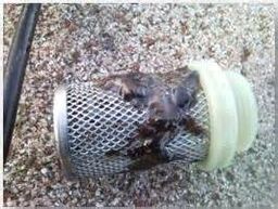
As I indicated at the end of May’s post , the data and other information that we collected during the RCA effort led to a hypothesis that dispenser slow-flow was caused by rust-particle accumulation on leak detector screens and that the particles detected on leak detector screens were primarily being delivered with the fuel (regular unleaded gasoline – RUL) supplied to the affected underground storage tanks (UST).

Commonly, during RCA efforts both actionable and non-actionable factors are discovered. An actionable factor is one over which a stakeholder has control. Conversely, a non-actionable factor is one over which a stakeholder does not have control. Within the fuel distribution channel, stakeholders at each stage have responsibility for and control of some factors but must rely on stakeholders either upstream or downstream for others.


For example, refiners are responsible for ensuring that products meet specifications as they leave the refinery tank farm (Figure 2a – whatever is needed to ensue product quality inside the refinery gate is actionable by refinery operators), they have little control over what happens to product once it is delivered to the pipeline (thus practices that ensure product quality after it leaves the refinery are non-actionable).


Pipeline operators (Figure 2b) are responsible for maintaining the lines through which product is transported and ensuring that products arrive at their intended destinations in the – typically distribution terminals in the U.S. – but are limited in what they can add to the product to protect it during transport.


Terminal operators can test incoming product to ensure it meets specifications before it is directed to designated tanks. They are also responsible for maintaining their tanks so that product integrity is preserved while it is at the terminal and remains in-specification at the rack (Figure 2c). Terminal and transport truck operators have a shared responsibility that product is in-specification when it is delivered to truck tank compartments (solid zone where Figures 2c and 2d overlap).


Tanker truck operators are also responsible for ensuring that tank compartments are clean (free of water, particulates, and residual product from previous loads). Additionally, truck operators (Figure 2d) are responsible for ensuring that tanker compartments are filled with the correct product and that correct product is delivered into retail and fleet operator tanks. They do not have any other control over product quality.


Finally, retail and fleet fueling site operators are responsible for the maintenance of their site, tanks, and dispensing equipment (Figure 2e).


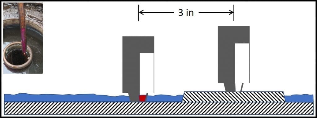
Regarding dispenser slow-flow issues, typically only factors inside the retail sites’ property lines are actionable (Figure 3 – copied from May’s post).

Fig 2. Limits of actionability at each stage of fuel product distribution system – a) refinery tank farm; b) pipeline; c) terminal tank farm; d) tanker truck; and e) retail or fleet fuel dispensing facility. Maroon shapes around photos reflect actionability limits at each stage of the system. Note that terminal and tanker truck operators share responsibility for ensuring that the correct, in-specification product is loaded into each tank compartment.

Fig 3. Dispenser slow-flow failure model.

As illustrated in Figure 3, the actions needed to prevent leak detector strainer fouling were not actionable by retail site operators. In this instance, we were fortunate in that the company whose retail sites were affected owned and operated the terminal that was supplying fuel to those sites.


A second RCA effort was undertaken to determine whether the rust particle issue at the retail sites was caused by actionable factors at the terminal. We determined that denitrifying bacteria were attacking the amine-carboxylate chemistry used as a transportation flow improver and corrosion inhibitor. This microbial activity:

– Created an ammonia odor emanating from the RLU gasoline bulk tanks,

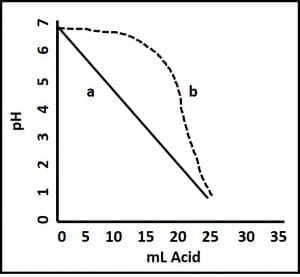
– Increased the RUL gasoline’s acid number, and

– Made the RUL gasoline slightly corrosive.


Although the rust particle load in each delivery was negligible (i.e., <0.05 %), the total amount of rust delivered added up quickly. If the rust particle load was 0.025 %, 4 kg (8.8 lb) of particles would be delivered with each 26.5 m3 (7,000 gal; 19,850 kg) fuel drop. The sites received an average of two deliveries per week (some sites received one delivery per week and others received more than one delivery per day). That translates to an average of 32 kg (70 lb) of particulates per month. Corrective action at the terminal eliminated denitrification in the RUL gasoline bulk tanks and reduced particulate loads in the RUL gasoline to <0.01 %.


Step 8. Institutionalize Lessons Learned

Although the retail site operators could not control the quality of the RUL gasoline they received, there were several actionable measures they could adopt.

1. Supplemented automatic tank gauge readings with weekly manual testing, using tank gauge sticks and water-finding paste. At sites with UST access at both the fill and turbine ends, manual gauging was performed at both ends.

2. Use a bacon bomb, bottom sampler to collect UST bottom samples once per month. Run ASTM Method D4176 Free Water and Particulate Contamination in Distillate Fuels (Visual Inspection Procedures) to determine whether particles were accumulating on UST bottoms. As for manual gauging, at sites with UST access at both the fill and turbine ends, bottom sampling was performed at both ends.

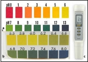
3. Evaluate particulate load for presence of rust particles by immersing a magnetic stir bar retriever into the sample bottle and examining the particle load on the retriever’s bottom (Figure 4).

4. Set bottoms-water upper control limit (UCL) at 0.64 cm (0.25 in) and have bottoms-water vacuumed out when they reach the UCL.

5. Set rust particle load UCL at Figure 4 score level 4 and have UST fuel polished when scores ≥4 are observed.

6. Test flow-rates at each dispenser weekly – reporting flow rate and totalizer reading. Compute gallons dispensed since previous flow-rate test. Maintain a process control chart of flow-rate versus gallons dispensed.

Fig 4. Qualitative rust particle test – a) magnetic stir bar retriever; b) attribute scores for rust particle loads on retriever bottom, ranging from 1 (negligible) to 5 (heavy).

These six actions were institutionalized as standard operating procedure (SOP) at each of the region’s retail sites. Site managers received the requited supplies, training on proper performance of each test, and instruction on the required record keeping. There has been no recurrence of premature slow-flow issues at any of the retail sites originally experiencing the problem.


Wrap Up

Although I used a particular case study to illustrate the general principles of RCA, these principles can be applied whenever adverse symptoms are observed. I have used this approach to successfully address a broad range of issues across many different chemical process industries. The keys to successful RCA include carefully defining the symptoms and taking a global, open-minded, multi-disciplinary approach to defining the cause-effect paths that might be contributing to the observed symptoms. Once a well-conceived cause-effect map has been created, the task of assessing relative contributions of individual factors becomes fairly obvious, even when the amount of actual data might be limited.


Bottom line: effective RCA addresses contributing causes rather than focusing only on measures that only address symptoms temporarily. In the fuel dispenser case study, retail site operators initially assumed that slow-flow was due to dispenser filter plugging. Moreover, they never checked to confrim that replacing dispenser filters affected flow-rates. This short-sighted approach to problem solving is remarkably common across many industries. To learn more about BCA’s approach to RCA, please contact me at fredp@biodeterioration-control.com.

FUEL & FUEL SYSTEM MICROBIOLOGY PART 28 – IS THE SULFUR IN HIGH SULFUR DIESEL TOXIC?

Diesel fuel biodeterioration is not affected by the fuel’s sulfur content.

There is a broadly embraced misperception about the relationship between diesel fuel’s sulfur content and its toxicity to microorganisms. This misperception is driven by two logical flaws.

Logical argument #1:

There has been an increase in the number of microbially contaminated fuel systems since the use of ultra-low-sulfur diesel (ULSD) became mandatory.

Therefore, microbial contamination in low sulfur diesel (LSD) and high sulfur diesel must have occurred less frequently than in currently does in ULSD.

Logical argument #2:

If argument #1 is valid, then the removed sulfur must have had a biostatic (ability to prevent microbes from growing) or biocidal effect.

“Get your facts first, and then you can distort them as much as you please.”

This quote was reportedly part of a session that Samuel Clemens (Mark Twain) has with young reporters sometime in the 1890s. More recently, in one of his many books on Zen, the philosopher Alan Watts, observed that humankind is unique in our uncanny ability to make precise and accurate observations only to use them to draw erroneous conclusions. Finally, in an earlier post I quoted Daniel Kahneman’s adage: “What you see is all there is.” (WYSIATI).

Logical argument #1 fallacies:

This argument assumes that the increased incidence of reports in a particular market sector (fuel retail) is equivalent to the increased incidence of microbial contamination in diesel fuels and fuel systems. But how do we know whether stakeholders are simply more aware of something that has been going on since diesel fuels were first used? The history of marine fuel oil biodeterioration that date back to the transitions from coal to oil and from burner oils to marine diesel fuel oil (more on this, in response to argument #2). Distillate aviation fuel biodeterioration has been recognized since the Korean War.

Additionally, the argument ignores various confounding factors (in statistics, a confounding factor is an unobserved variable that affects observed variables: in our case sulfur concentration and biodeterioration are observed variables. Before concluding that removing sulfur made diesel fuel more vulnerable to biodeterioration consider these four confounding factors (there are others, but these five illustrate the concept):

  • Hydrotreatment to remove sulfur also removes aromatic compounds – especially high molecular weight, toxic, polynuclear aromatic compounds.
  • During the past three decades, the fuel distribution infrastructure has evolved from vertically integrated control (the refiner controlled all stages from refinery to retail site) to fungible (common pipelines transport products from refinery tank farms to terminals from which independent and branded retailers draw product from tanks that can that can be mixtures of product from numerous refineries – >100 refineries produce product that is stored in in New Jersey terminal tanks). Fungible product comingling means that cradle to grave product stewardship is more complex than it was historically.
  • Product transport from terminals to fleet operators and retailers is typically done my third-party transport companies. Switch-loading (a given tank compartment can carry gasoline on one trip and diesel on the next) is occurring more frequently. The probability of cross-contamination between two fuel-grades is a hotly debated issue at present.
  • Although the trend is beginning to reverse itself, between 1990 and 2010, total diesel storage capacity shrunk annually as product demand grew. Consequently, residence time in terminal storage tanks has decreased. Although best practice is to give water and particulates time to settle before drawing product from a tank to the fueling rack, product demand can inspire terminal operators to begin drawing product early. Consequently, any water, particulates, or both that have not settled to below the suction zone will be transported with the fuel.
  • Dispensing system technology has become more sophisticated. Systems that might not have be affected historically, are now failing – primarily due to corrosion damage. As a microbiologist, I’d like to think that all fuel system corrosion is microbiologically influenced corrosion (MIC). However, if ethanol enters diesel fuel systems (either because of switch loading or vapor recovery unit vapor comingling) it can be chemically oxidized to acetic acid. Therefore, unless other low molecular weight (4 to 6-carbon) organic acids are also present, high concentrations of acetic acid in fuel-associated water is likely to be a symptom of chemical – not microbial – activity.

Logical argument #2 fallacies:

This argument is built on argument #1’s house of cards. It falls apart if the statement: “There has been an increase in the number of microbially contaminated fuel systems since the use of ultra-low-sulfur diesel (ULSD) became mandatory.” is false. As noted above, increased incidence and increased reports are two very different concepts.

To illustrate this point, consider the respiratory disease, legionellosis. The disease was given its name because the first recognized outbreak was among American Legion members attending a convention at the Bellevue-Strafford Hotel, in Philadelphia. It is beyond improbable that the bacterium that causes legionellosis – Legionella pneumophila – came into existence in 1976. However, in late July and early August 1976, after 221 American Legion convention attendees developed pneumonia-like symptoms, and 34 of the patients died, the medical establishment (physicians and epidemiologists) took note. It took a couple of years to figure out how to culture L. pneumophila, and there was wild speculation regarding the likely relationship between environmental conditions and the microorganism’s ability to grow. Forty years down the road, we know that L. pneumophila is ubiquitous – it can be found in many different environments where biofilms develop (relax – none yet recovered from fuel systems; but don’t relax too much – shower-head aerator screens tend teem with L. pneumophila). The good news is that only immunosuppressed individuals tend to develop the legionellosis.

What does this have to do with the relationship between sulfur concentration in fuel and biodeterioration risk? In both cases, the microbes causing the symptoms have been around for a long time. In the health sector, for centuries (if not millennia) L. pneumophila has caused an unknown percentage of all pneumonia cases, but it was never identified because there had never been (i.e., since the advent of modern medical microbiology, immunology, and epidemiology) such a large number of folks getting sick at the same time and place. Similarly, fuel biodeterioration was well known from the earliest days of gasoline and diesel production. However, there was no database documenting each biodeterioration event.

Prior to 2012 the upper limit for sulfur in marine diesel was 4.5 %. Before 1986, on-highway diesel typically had 0.1 % to 0.5 % (by volume) sulfur. If the sulfur in these historical fuels had been biostatic, fuel biodeterioration would have not occurred until ULSD came onto the market. Filter plugging on ships and aircraft had a more serious impact than filter plugging on dispensers, locomotives, and other land-based diesel fuel systems. However, efforts to control microbial contamination in the marine and aviation sectors were not general knowledge among fuel retailers and fleet operators. Ironically – because they ignored the biocidal effect of tetraethyl lead – folks were convinced that gasoline was too toxic to support microbial growth and that only diesel fuels and fuel systems were affected.

Despite all of this, isn’t it fair to say that ULSD biodeterioration is more pervasive than that of diesel grades with greater sulfur concentrations? My answer is: Not necessarily. There are no hard statistics on the average number of ULSD biodeterioration incidents per year since 1986 and there are certainly no reliable statistics for the decades before the switch to ULSD (or in off-highway systems using low or high sulfur diesel). The assessment that the incidence rate has increased since ULSD replaced other fuel grades for on-highway use is purely subjective. One more time: increased awareness (as in the case of legionellosis) is not the same as increased incidence. The switch to ULSD and biodiesel blends was highly visible to the industry. From the outset, stakeholders wanted to know what the change might do to their systems. Consequently, they now notice damage more quickly than they had in the past. Okay, this is an optimistic statement. In two recent fuel quality surveys, sites originally identified as control sites (no reported problems) had more microbial contamination and corrosion than he problem sites. In the more recent, US EPA-sponsored study, operators were unaware of any problems at 87 % of the moderately to heavily corroded sites.

The Science:

There is no question that some organosulfur compounds are biocidal. For example, two of the few fuel-treatment biocides are mixtures of organosulfur compounds:

CIT/MIT (also referred to as CMIT): 5-Chloro-2-methyl-3(2H)-isothiazolone + 2-methyl-3(2H)-isothiazolone (isothiazolinones are ring structured molecules with the chemical formula: C₃H₃NOS).

MECT: 2-(Thiocyanomethylthio)benzothiazole + Methylene bis(thiocyanate) (the thio in each molecule’s name indicates that they are organosulfur compounds)

However, sulfur is one of the five primary elements (the other four are: carbon, hydrogen, nitrogen, and oxygen) on which all life depends.

Studies on fuel biodegradability have shown that the aromatic content, rather than the sulfur content is a primary factor affecting diesel biodegradability. Regardless of sulfur concentration, fuels with higher aromatic concentrations or more complex aromatic compounds biodegrade more slowly than more severely hydrotreated fuels from which aromatics have been substantially removed. The same hydrotreating process that removes sulfur also reduces fuel’s aromatic content. Note that although there are no aromatic biocides approved for fuel treatment, there are numerous aromatic biocides approved for other applications.

    Bottom line:

If ULSD fuels are more susceptible than higher sulfur content fuels are to biodeterioration, it is due to the reduced concentration of complex, toxic polynuclear aromatic compounds – not because of sulfur’s inherent toxicity.

FUEL & FUEL SYSTEM MICROBIOLOGY PART 24 – PETROLEUM EQUIPMENT INSTITUTE’S 2018 CONVENTION

The Petroleum Equipment Institute (PEI) held its 2018 convention at the Las Vegas Convention Center from 07 to 10 October 2018. As usual, the PEI convention was held in conjunction with the much larger National Association of Convenience Store (NACS) convention. Today, I’ll focus on a few items that are particularly relevant to fuel and fuel system microbiology. I’m not going to attempt to provide anything approaching an overview of the entire convention. Instead I’ll report and discuss a few statements I heard from speakers during PEI’s Tuesday 09 October education sessions.

Regulatory issues

EPA Regulatory Update – Carolyn Hoskinson, Director of EPA’s Office of Underground Storage Tanks (OUST) and several members of her staff spoke to the current state of affairs regarding UST regulations. Tony Raia reported that with the 13 October 2018 compliance deadline looming, 32 states had updated their UST regulations to harmonize them with the 2015 updated US EPA regulations. Tony identified five state categories:
1. State Program Approval (SPA) States that have completed their updates and which are now in full compliance
2. Non-SPA States that have completed their updates to comply with the 2015 regulations
3. SPA States that have delayed revising their state regulations
4. SPA States that have updates in progress
5. Non-SPA States that have not yet updated their regulations per the US EPA 2015 regulations.
Bottom line is that we are entering a period during which there will be some confusion over compliance.

U.S. EPA UST Enforcement – Mark Barolo – the US EPA OUST official responsible for enforcement – noted that in nearly all cases, individual States were responsible for enforcement. Recognizing the confusion, Mark opined that inspectors were going to address violations on a case-by-case basis. Generally speaking, retailers who had been incompliance, had the required documentation, and demonstrated that they were making good-faith efforts to ensure that they remained in compliance, would experience less enforcement grief than those who have not. Mark’s colleague, Cho Yi Risher noted that the regulations do not prescribe the time permitted for site owners to repair or replace non-compliant equipment. Moreover, the inspections required by the 2015 regulations identify non-compliant equipment. There is no incentive for owners to institute predictive maintenance programs (see my 16 January 2017 post) that would detect failure trends before equipment became non-compliant.

Failure to detect uncontrolled microbial contamination and biodeterioration before they cause valves to seize or tanks and lines to leak is a false economy. A few pennies saved during regulation-mandated inspections can lead to remediation expenses in excess of $0.5 million.
Although for some of us, it’s hard to believe that the UST installed in 1987 – in compliance with the original UST regulations – are now beyond their 30-year warranty life. Discussion during the session’s question and answer period indicated that all stakeholders shared a common interest in ensuring that sites with tanks that were more than 30-years old would be able to continue to operate. I anticipate seeing articles to this issue in PEI Journal in the coming months.

Fuel Quality and Corrosion
Scott Boorse – PEI’s Technical Program Manager; recently retired from a major fuel retailer – made several observations that validated much of what I’ve been discussing in Fuel Microbiology What’s New posts. He suggested that in his experience, 100 % of all retail site fuel systems had some corrosion. He attributed much of this corrosion to the bacterial genus Acetobacter converting ethanol to acetic acid. I am convinced that most of the headspace and spill containment well acid production comes form chemical oxidation of ethanol to acetic acid. Microbes are involved in an estimated 50 % of all system corrosion issues, but – as I’ve written previously – microbes produce a variety of organic acids. These acids can react with chloride, sulfate, and nitrate in fuel-associated water to form organic bases (or salts) and strong, highly corrosive, inorganic acids – hydrochloric, sulfuric, and nitric acids, respectively. Still, Scott was on spot suggesting that UST system corrosion was much more wide-spread than most stakeholders realize.

Rebbeca Moore – GM and chair of the automotive industry’s Top Tier Detergent Gasoline and Diesel Fuel consortia – discussed the importance of fuel quality on engine performance. Top Tier is an auto industry sponsored compliance program intended to go beyond ASTM product specifications typically cited in state regulations. I’ll steer clear of the perennial debates between engine manufactures and petroleum producers that enliven our semi-annual ASTM D02 (Petroleum Products) subcommittee A (Gasoline and Oxygenated Fuels) and E (Burner, Diesel, Non-Aviation Gas Turbine, and Marine Fuels), but Rebbeca made an important point. ASTM specifications are often misused. They are meant to indicate whether a product (i.e., fuel) is fit for use at a single point and place in time (i.e., when and where the sample was collected). The petroleum industry’s infrastructure is vast and complex. Moreover, product ages (if it didn’t it wouldn’t combust so well in engines). Specification tests provide little information about how the product will age during storage.
Rebbeca illustrated the dilemma by listing the typical components of 7,500 gal of in-specification ULSD delivered to UST:
• 1 cup of dirt
• 1 to 2 gallons of water
• Up to 325 gallons of FAME (B5 ULSD is now included in ASTM Specification D975 Diesel Fuel Oils)
• 1 gallon of glycerin
• 5 to 40 gallons of additives
At sites that receive frequent deliveries, these trace amounts of dirt and water add up! Not surprisingly, along with measures that are outside the retail site or fleet owner’s control, Rebecca recommended more aggressive water removal and better dispenser filtration (there is an ongoing debate among stakeholders with some recommending that all dispensers have 5.0 µm, water absorbing filters and others arguing for 100 µm particulate filters). I share Rebecca’s view that all dispensers should have 5.0 µm, water absorbing filters. Marketers who are focused only on low rates and not product quality have argued for eliminating the filtration requirement completely.

Ryan Haerer – of US EPA’s OUST (https://www.epa.gov/ust) – wrapped up the session, sharing a few notable points. First, Ryan reminded attendees that UST regulations apply only to system components that are in contact with the soil. The US EPA does not regulate the condition of internal components that are not in direct contact with the soil (for example, submerged turbine pumps – STP – and their associated hardware). He also explained that under the UST regulations, there is a requirement that system components be compatible with the substance stored. This is likely to become interesting as new products (for example, E15 gasoline or substitution of ethanol with isobutyl alcohol) are introduced into the commercial fuel infrastructure – here I’m using interesting – in the same way it is used in of the phrase: “May you live in interesting times.” (Austen Chamberlain – British Foreign Secretary, 1924 to 1929 wrote that he had been told that this was an ancient Chinese curse, but his claim has never been verified).

Bringing it home

At this point we are enjoying an interesting paradox. Regulators, insurers, and an increasing number of retailers recognize that waiting until fuel systems fail is a problem. However, the system largely provides incentives for site owners to wait until failures have occurred. After failure, insurance covers component replacement costs. In many states, superfund monies cover remediation costs. When site owners invest in predictive maintenance, they only see the costs. Although there are benefits – not the least of which is customer satisfaction and a positive corporate image – they are intangible. How do we break the paradox?

Please share your thoughts on this issue with me at fredp@biodeterioration-control.com. I’ll compile comments and post them anonymously as a future What’s New column.

FUEL & FUEL SYSTEM MICROBIOLOGY PART 20 – PREVENTING MICROBIAL DAMAGE TO FUEL SYSTEMS PART 2; WATER BITS


Fig 1. From Rime of the Ancient Mariner, Samuel Taylor Coleridge, 1798

Water, water everywhere…

Samuel Coleridge’s infamous mariner paid dearly for having killed an albatross (figure 1). Do fuel quality managers and personnel responsible for fuel system integrity pay dearly for underestimating the ability of small (<1 oz; 30 mL) pools of fuel-associated-water left behind after water has been nominally purged from a fuel tank? A water bit is any small volume of water that remains in a fuel tank after dewatering (my personal, technical definition).
In Part 20, I wrote: “No water means no bugs. Is it as easy as all that?” I also explained why the short answer to the question was: “No.” For emphasis, I’ll again share figure 3 from Part 20 (figure 2, here):


Fig 2. Scale: how 2 mm of water appears to a bacterial cell.

A – a 6’6” tall man standing at the base of Mt. Kilimanjaro; B- a bacterial cell “standing” in a pool of water that is >2 mm deep; the ratios between the height of Mt. Kilimanjaro and the man in A, and between the depth of the pool of water and the bacterial cell in B are the approximately the same.

What can we do about these traces of water?
I confess that I am not a big fan of dispersants. When water dispersants are used routinely as fuel additives, the dispersed water can act as a corrosive agent; damaging engine components. However, when used to complete the job started by draining or vacuuming most of the free-water out of a tank, dispersants can be quite effective.
Figure 3 illustrates how dispersants work. Most dispersants are organic molecules that have a polar (charged; water-soluble) head and a non-polar (non-charged; fuel-soluble) tail. When added to fuel over water (figure 3b), they move towards anywhere where fuel contacts water (figure 3c) and trap tiny (typically <1 µm; 0.0004 in dia) fuel droplets. The fuel “sees” only the dispersant’s non-polar tails, so the droplets disperse uniformly throughout the fuel (figure 3d). The dispersed droplets (micelles) get transported with the fuel and evaporate during combustion in the engine cylinder.


Fig 3. Dispersant action: a) fuel over bottoms-water; b) dispersant added to fuel – inset shows dispersant molecule with polar head and non-polar tail; c) dispersant heads and tails align in water an fuel phases, respectively; d) dispersants form micelles with water droplet trapped in center; typical droplet size is < 1 μm dia.
The use of dispersants is controversial. Dispersant manufacturers and marketers focus on dispersant effectiveness in keeping free-water from accumulating in fuel systems. Moreover, under most circumstances, microbes are unlikely to make use of water trapped within dispersant micelles. Conversely, engine manufacturers focus on the potential for dispersed water to corrode and erode injector nozzles; particularly on modern, high-pressure, common-rail diesel engines. Interestingly, there is at least one additive manufacturer that has tried to promote water-emulsion diesel fuels – diesel with a dispersant that enables the fuel to hold as much as 25 % water. As a microbiologist, I was looking forward to investigating microbial contamination problems in systems that handled 25-75 water-in-diesel blends. But that’s another discussion.
In my next blog, I’ll focus on fuel treatment biocides. In the meantime, if you have questions or comments about today’s post, please contact me at fredp@biodeterioration-control.com.

Disclaimer:
Microbes are ubiquitous. There are extraordinarily few habitats on earth where thriving, microbial communities have not been detected. In practical terms, this means that it is unlikely that operators will ever have a completely sterile fuel system or that they will reduce their fuel system biodeterioration risk to zero. Biodeterioration can still occur in the best maintained fuel systems. However, the risk of it occurring in an inadequately maintained system is much more likely.

FUEL & FUEL SYSTEM MICROBIOLOGY PART 17 –TEST METHODS – GENETIC TESTING

In today’s blog, I’ll cover the lastest family of microbiology methods used for testing fuels & fuel associated water. These methods fall under the category genomics – the study of genes. Warning: genetic testing is more technically complex than the methods I’ve described in recent posts. I’ll do my best to keep the language as simple as possible.

Genetic methods have evolved substantially over the past 30 years. They all depend on the polymerase chain reaction (PCR); first reported in 1983. The common steps of all PCR methods include:

   1) Genetic material (deoxyribonucleic acid – DNA) extraction (fig 1).
   2) Heating to separation of the two strands of DNA’s double helix (fig 2) into two single-strands.
   3) Cooling and using an enzyme – polymerase – to convert each single strand back into double stranded DNA (fig 3).
   4) Repeating steps 2 and 3 until there are millions of copies of each of the DNA originally extracted in step 1.
   5) Using analytical tools to: identify the different types of DNA that were extracted from the original sample in step 1.

Fig 1. Bacterial cell lysing and ejecting its cytoplasm

Fig 2. a) DNA molecule ; b) section of DNA being denatured to two single strands.

Fig 3. Denatured DNA (left) coupled with primer and reacted with DNA polymerase to form two new double helices.

When PCR methods were first developed in the mid-1980s, DNA was extracted from colonies that had developed on nutrient agar plates (see Part 12 and fig 4). Early PCR testing revolutionized microbial taxonomy. Microbes that seemed to be closely related because of their appearance and nutrient preferences turned out to be quite distant genetic relatives. Conversely, some microbes that had historically been classified as being members of different groups, were discovered to be nearly identical genetically. However, PCR could only be used to identify microbes that formed colonies.

Fig 4. Bacterial colonies on nutrient agar.

In the 1990s quantitative-PCR (qPCR) methods were developed. In qPCR, messenger-RNA (mRNA) is extracted and used to synthesize complimentary-DNA (cDNA). The PCR process then continues as described in steps 2 through 5. The RNA used for qPCR is typically tagged with a fluorescent dye. A fluorometer is used to measure the DNA concentration as a function of time during repeated cycles of heating and annealing (steps 2 and 3). As shown in fig 5, the time required for the fluorescence to reach a threshold value, can be used to compute the amount of mRNA that was originally extracted from the sample. This, in turn provides an accurate estimate of the population density (i.e., cells/mL) in the sample.

Fig 5. DNA amplification curves: delta Rn is the amount of fluorescence detected and ct is the threshold delta Rn used to compute the DNA concentration in the original sample. The five curves show that the number of PCR cycles needed to reach ct increases as the original DNA concentration decreases.

Four molecules (nucleotides) make up the genetic code (adenosine – A, cytosine – C, guanine – G, and thiamine – T). Each three-nucleotide sequence is the code for a specific amino acid. Thus, long strings of three-letter messages specify the amino acid sequence of enzymes – the cell’s machinery for carrying out all of life’s processes. The total genome of each type of cell (operational taxonomic unit – OTU) is unique. Because each of the four nucleotides – A, C, G, and T – has a unique electrical charge, each OTU’s DNA has a unique net electrical charge. Using a technique called gel electrophoresis, after amplification (step 5) analysts can separate and isolate each type of DNA that was recovered from the original sample (fig 6). They can then sequence the genes and attempt to match the sample’s DNA against a DNA library. The result is a taxonomic profile of the microbes that were present in the original sample.

Fig 6. DNA profiling using gel electrophoresis: a) schematic illustration of process ; b) photograph of gel.

In earlier posts, I’ve referred to Donald Rumsfeld’s “unknown unknowns.” Although qPCR and, the more recently variation called next generation sequencing – NGS, is a powerful tool for studying microbial communities in fuel systems, it is probably not the last word in microbiology testing. True, qPCR detects many types of microbes that are undetectable by historically used culture methods. However, extracting DNA or RNA from cells is as much art as science. Genetic material that isn’t extracted isn’t detected. Additionally, qPCR testing depends on the use of primers – short sections of mRNA selected to either be universal (i.e., include a section of A, C, G, T basis that are believed to be present in all bacteria) or specific (i.e., include a section of genetic coding that is unique to a microbe of specific interest). Consequently, researchers are on a steep learning curve about how to select primers. As task force within ASTM D02.14 has just restarted work on a qPCR standard test method for fuels and fuel associated water. The last attempt stalled when participants could not agree on a consensus DNA extraction protocol. As the new task force makes progress I provide readers with updates. The goal is to develop a method that non-technical folks will be able to use.

In the meantime, please contact me at fredp@biodeterioration-control.com you’d like to learn more about fuel system microbiology or microbiological contamination control.

Footnotes:

Source: http://www.newswise.com/images/uploads/2013/01/9/lysis_cover.jpg.
Source: http://www-nmr.cabm.rutgers.edu/photogallery/proteins/gif/dna.gif.
Source: https://laboratoryinfo.com/wp-content/uploads/2015/07/Polymerase_chain_reaction.svg_.png.
Source: https://www.microbiologyinpictures.com/bacteria-photos/escherichia-coli-photos/e.-coli-staphylococcu-aureus-colonie.jpg.
Source: https://media.nature.com/full/nature-assets/leu/journal/v17/n6/images/2402922f5.jpg.
Source: http://science.halleyhosting.com/sci/ibbio/biotech/pics/electrophoresisnotes.gif.
Source: https://78.media.tumblr.com/tumblr_lwthmyKO441qzcf71o1_500.gif.

FUEL & FUEL SYSTEM MICROBIOLOGY PART 15 – TEST METHODS – HOW DO WE DETECT BUGS ON SURFACES?

In my August post (https://biodeterioration-control.com/microbial-damage-fuel-systems-hard-detect-part-14-test-methods-still-microbiological-tests/), I discussed using ASTM D7687 to quantify microbial loads (AKA bioburdens) in liquid samples – fuels and fuel associated water. This post will focus on surface samples.

Generally speaking, microbes tend to be most abundant on surfaces. By some estimates, in any given system, for every microbe floating in the bulk fluid, there are 1,000 to 1,000,000 growing on surfaces. These surface microbes are invariably part of biofilm communities. I’ll discuss biofilms in more detail in a future post. For now, it is sufficient to understand that biofilms are slime-encased microbial communities growing on surfaces (fig 1). It is much easier to grab a fluid sample than a surface sample. Consequently, most fuel system samples – even those intended for microbiology testing – are fluids. However, there are a few fuel system surfaces that can be sampled relatively easily.


Fig 1. Scanning electron micrograph of a mature biofilm. Note its structural complexity. Source http://drandreastevens.com/wp-content/uploads/2016/02/Biofilm-Photo.png


Fig 2. Automatic tank gauge, water float showing slime accumulation (right) and swabbed area (left).

Biofilms tend to develop on automatic tank gauge (ATG) water floats (fig 2). The left side of the water float shown in figure 2 has been swabbed. The right side shows the undisturbed deposit. This deposit includes microbes, their slime, and metal fins (i.e. rust). Most often, I use a swab to collect a sample from a premeasured surface area. If the deposit is > 2 mm (1/8 in) thick, I use a spatula to collect the sample.

The second location I routinely check for microbial contamination is the filter. Figure 3a shows a 76 cm (30 in) filter cartridge. It was one of 16 cartridges in a high-capacity filter housing. However, except for its length, the 76 cm cartridge does not look very different from the filter element inside a typical fuel dispenser filter (fig 3b). To test the filter element for microbial contamination, I first inspect the element visually; looking for slime accumulations or discolored zones. For larger filters, I use an alcohol-disinfected forceps and scissors to cut out a section ( 4 cm x 4 cm; fig 3c), and from that cut out a 1 cm x 2 cm piece of filter medium (fig 3d). For dispenser filters, I cut out a 1 cm x 2 cm piece directly. This is my specimen.

If a dispenser has a screen (fig 4), upstream of the filter I collect either a swab or spatula sample just as I would from the ATG water float.


Fig 3. Fuel filter sampling: a) 60 cm filter element from high-capacity housing; b) dispenser filter element; c) section of filter media taken from element shown in fig 3a; d) 1 cm x 2 cm specimen taken from section shown in fig 3c.


Fig 4. Fuel dispenser prefilter screen partially covered with slime.

Once I’ve collected my surface sample I run LuminUltra Technologies, Ltd, Deposit and Surface Analysis (DSA) test (for more information about the DSA method visit https://www.luminultra.com/dsa/; for a video demonstration, visit https://www.youtube.com/watch?v=VEhpbvtej3E). The method provides me with a rapid, quantitative measure of the bioburden on these fuel system surfaces.

Total ATP concentration ([tATP]) <100 pg/cm2 indicates negligible surface contamination. [tATP] between 100 pg/cm2 and 1,000 pg/cm2 indicates moderate contamination (it’s time for maintenance action). [tATP] ≥ 1,000 pg/cm2 signals that prompt corrective action is needed! If you have weighed out samples, the [tATP] per g threshold levels are the same as those for [tATP] per cm2.

If you’d like to learn more about fuel system surface microbiology, please contact me at fredp@biodeterioration-control.com.

FUEL & FUEL SYSTEM MICROBIOLOGY PART 11 –TEST METHODS – BOTTOM SAMPLE CHEMICAL TESTS

We are progressing from test methods that do not require any equipment (other the tools you need for sample collection) to those that require increasingly expensive tools. You can complete basic gross observations by relying on your eyes and nose. The physical tests I suggested in Part 10 require simple tools; including a magnetic stirring bar retriever, disposable syringes, filter pads and in-line filter holders. In this blog, I’ll discuss a couple of simple chemical tests. However, with one exception, the devices used to run these tests cost a few hundred dollars. This means that under most circumstances, I’ll be writing about tools that condition monitoring service teams, rather than individual site owners, should have on hand.

Water paste is the exception I was referring to above. I hope that if you are reading this blog, you are familiar with water paste and how to use it to detect bottoms-water. For readers who are unfamiliar with it, water paste is a thick substance that can be applied to the bottom of a sounding stick or gauge bob (fig 1). Note that if the gauging stick does not contact the tank’s actual bottom, water that’s present might go undetected.

Fig 1. Using water paste to detect bottoms-water. Left inset: gauging stick with bottom 6 inches coated with paste. The paste had been white, but had turned purple after having been lowered to the tank bottom and removed. The purple color change indicated that there were at least 6 inches of bottoms-water in the tank. Many UST have strike-plates under the fill-line. In this schematic, the UST has 0.25 inches of water. Because the strike-plate is 0.5 inches thick, gauging fails to detect the water. Had the stick contacted the UST bottom, just beyond the strike plate, the paste would have shown that 0.25 inches of water were present.

Why do I list water-paste use as a chemical test? Because the color change is a chemical reaction.  Also, if there isn’t any bottoms-water in your bottom sample, you cannot run either of the other two tests I’m covering in this post.

Point of nostalgic disclosure: the chemical tests that I am about to describe used to be more useful than they are now. Many fuel additives can move from fuel into water. This process is called partitioning. Let’s say that a particular additive is 100% soluble in fuel and 20% soluble in water. Whenever a fuel tank has any free-water, the additive will partition into the water until its concentration in the water is 20%. Keep in mind that in a UST with 7,000 gal of fuel and 70 gal of water (yes, that’s a lot of water!) the fuel to water ratio is 700 to 1. This means that even though the additive’s concentration is 20% in the bottoms-water, only an immeasurably small amount of the additive has partitioned out of the fuel. The fuel’s chemistry isn’t affected, but the water’s chemistry is. Let’s see how this affects pH and total dissolved solids (TDS).

pH measurement provides an indication of an aqueous solution’s acidity.  pH ranges from 0 to 14; with pH = 7 being neutral, pH <7 being acidic, and pH >7 being alkaline. The lower a solution’s pH, the more acidic it is. For example, the pH of stomach acid is in the 1.5 to 3.5 range (it’s essentially hydrochloric acid). Conversely, the higher the pH of a fluid, the more alkaline it i(bleach’s pH = 12). Historically, bottoms-water pH <6 was a good indicator of microbiological activity (microbes produce a variety of acids).  Although pH <6 still suggests microbiological activity, some fuel additives act as buffers – they prevent pH change.  Fig 2 illustrates the difference between adding acid to unbuffered water and adding it to buffered water.  The pH eventually falls in both cases, but when buffer is present, it takes substantially more acid to get to the same pH.  This means that in today’s fuel systems, pH drop is a later problem indicator than it was in the days before there were as many additives that partitioned into the water.

Fig 2. Buffer effect. Acid is added to two aqueous fluids; both with pH = 6.8. Fluid a is unbuffered. There is a straight-line relationship between the volume of acid added to the sample and its pH. Fluid b is buffered. Its pH does not begin to change appreciably until after 12 mL of acid have been added.

The easiest way to measure bottoms-water pH is to use pH paper (available from scientific supply distributors). Transfer a few mL of bottoms-water into a clean test tube or other small container. Dip a pH test strip into the water. After a few seconds, compare the color on the test strip against the color comparison chart provided with the test strips (fig 3). Generally, it’s sufficient to use tests trips that give whole pH unit results (fig 3a). If you want more precision, you can run a second test using pH paper that detects 0.2 pH differences (fig 3b). Digital pH meters (fig 3c) are generally more precise (reading to 0.01 pH units) than indicator strips. However, meters are more expensive than disposable test strips. Additionally, if meters are not kept clean and calibrated, they can give you precise, but inaccurate results.

Fig 3. pH test kits: a) broad range (pH 0 to 13), pH test strips with 1 pH unit precision; b) narrow range pH test strips with 0.2 pH unit precision; c) hand-held pH meter.

The final chemical test I’ll discuss today is TDS. As the name implies, TDS include all dissolved chemicals (organic and inorganic) in bottoms-water. Before the late 1990’s, typical gasoline bottoms-water TDS were in the 150 mg L-1 to 250 mg L-1 range and diesel fuel bottoms-water TDS were in the 250 mg L-1 to 500 mg L-1 range. High TDS concentrations would signal the presence of dissolved metals (corrosion byproducts), microbes and their metabolites, or both. However, the increased use of fuel additives that can partition into the water has translated into TDS >2g L-1 in both gasoline and diesel fuel bottoms-water. This high background TDS concentration can mask the contribution of microbes and corrosion to the total. There is a work-around, but the details are beyond the scope of this blog post.

TDS can be measured by weighing the residue that’s left behind after the fluid has evaporated away. However, TDS is directly related to conductivity (the ability of a material to carry an electrical current). The easiest way to measure TDS is to use a handheld meter (fig 4). Most meters offer the option of showing either conductivity (µS cm-1) or TDS (mg L-1).

Fig 4. Conductivity meter.

If you collected a good sample, by the time you have collected water level, pH, and TDS data, you know quite a bit about the condition of the fluids in your tank. You are at the “if it walks like a duck and quacks like a duck…” point of your field testing effort. You should be 90% certain of whether you have uncontrolled microbiological contamination (MC) in your system. Final confirmation depends on microbiological test results. I’ll begin to discuss these in my next post. Of course, if you want to learn more now, please send me an email at fredp@biodeterioration-control.com.

FUEL & FUEL SYSTEM MICROBIOLOGY PART 3 – TESTING

.

How much of the total microbial load each type of test detects.


I’m starting this post with an illustration from one of my recent presentations (click on the image to enlarge it). The quote is from Daniel Kahneman’s book: Thinking, Fast and Slow. It reminds us of how often our perceptions are much more limited than we realize. Let’s turn to the circles to the right of the quote.

(more…)

FUEL & FUEL SYSTEM MICROBIOLOGY PART 2 – SAMPLING

In his 1967 book, “The Use of Lateral Thinking” Edward di Bono introduced the concept identified in the book’s title. He contrasted “lateral thinking” against “linear thinking” and argued that successful resolution of any challenge required both types of thinking. What does this have to do with detecting microbes in fuel systems. Standard Practices, such as PEI’s RP900 “Recommended Practices for the Inspection and Maintenance of UST Systems”, are examples of excellent linear thinking. They prescribe a series of steps for performing UST system condition monitoring. Similarly, ASTM D4057 “Practice for Manual Sampling of Petroleum and Petroleum Products” provide a wonderful, linear sequence of steps for collecting fuel samples. Neither of these documents promotes lateral thinking. RP900 is great at detecting component failures once they occur. Similarly, D4057 is great for obtaining samples on which to run tests to determine whether the product is in specification. In contrast, ASTM D7464 “Practice for Manual Sampling of Liquid Fuels, Associated Materials and Fuel System Components for Microbiological Testing” encourages lateral thinking. It encourages users to ask: “what do I intend to do with my sample” and “if I want to detect microbial contamination, what kind of sample do I need to collect; from where should I collect that sample?”
Samples collected per D4057 are unlikely to contain microbes. Consequently, they are not the samples on which it makes any sense to test for microbial contamination. This is the number one reason microbial contamination in fuel systems remains undetected even after the bugs have caused component failure. Microbes need free-water to thrive. Free-water accumulates as condensate on tank surfaces – particularly in the headspace, above product, and on the tank bottom, below product. A substantial volume of free-water is also trapped within slime that accumulates on tank walls. Linear thinking guides us to collecting UST bottom-samples from fill-lines. Lateral thinking helps us to consider alternative sampling points and sample types. If you are interested in learning more about sample collection for microbiological testing, contact me by phone (609.716.0200) or email (fredp@biodeterioration-control.com). In my next blog post, I’ll discuss microbiological test methods.

FUEL & FUEL SYSTEM MICROBIOLOGY PART 1 – THE VALUE PROPOSITION.

When I ask petroleum retailers if they have microbial problems in their fuel systems, almost always, the answer is: “No!”. After reading EPA’s recent report – Investigation of Corrosion Influencing Factors in Underground Storage Tanks with Ultra Low Sulfur Diesel Service – I felt better; sort of. The report’s Executive Summary states: “We observed 83 percent of the inspected tanks had moderate or severe metal corrosion. Prior to our research inspections, less than 25 percent of owners reported knowledge of corrosion in their UST systems.” It also observes: “Our research suggests that MIC is likely involved in the moderate or severe internal corrosion in USTs storing diesel.” For the uninitiated, MIC stands for “microbiologically influenced corrosion”.
Now think about this. Regardless of whether UST were fiber-reinforced polymer (FRP) or steel, the vast majority of UST tested had moderate to severe corrosion. Yet only 25% of site owners were aware of the problem. How is this possible? Perhaps we find one explanation in two, September 2016 PMAA Journal articles. Both report how PMAA leadership convinced the U.S. EPA to roll back their initial full set of routine system inspection items that were to be required under the 2015 revisions to the UST Regulations (40 CFR part 280). Interestingly, both articles focus only on the apparent savings site owners will realize. Neither article mentions that the repair and site remediation costs associated with fuel system leaks or failures: $250,000 to $500,000. Note that these estimates do not include revenues lost during site repair. Now let’s consider how many years of more thorough site inspection and condition monitoring one could get for a system failure that only cost $250,000. The PMAA Journal articles suggest a savings of approximately $4000/year/site. That translates into >62 years of more thorough condition monitoring that would reduce the risk of failure substantially. I think that it is particularly noteworthy that the PMAA Journal articles indicate that “PMAA is helping to revise the Petroleum Equipment Institute’s RP-900” in order to reduce the thoroughness and frequency of the walk through inspections detailed in RP-900. Is this a penny wise, pound foolish strategy? In my next post, I’ll discuss the problems with current fuel retail condition monitoring programs. Spoiler alert: I won’t be arguing that they are too burdensome or expensive.

OUR SERVICES

  • Consulting Services
  • Condition Monitoring
  • Microbial Audits
  • Training and Education
  • Biocide Market Opportunity Analysis
  • Antimicrobial Pesticide Selection

REQUEST INFORMATION


    captcha