Archive for the ‘Fuel Microbiology’ Category

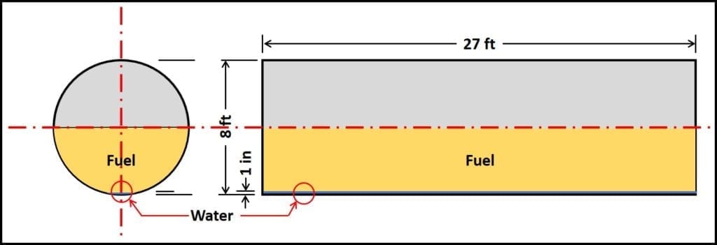
MICROBIOLOGY FOR THE UNINITIATED – PART 1: WHAT ARE MICROORGANISMS AND WHY SHOULD WE CARE?

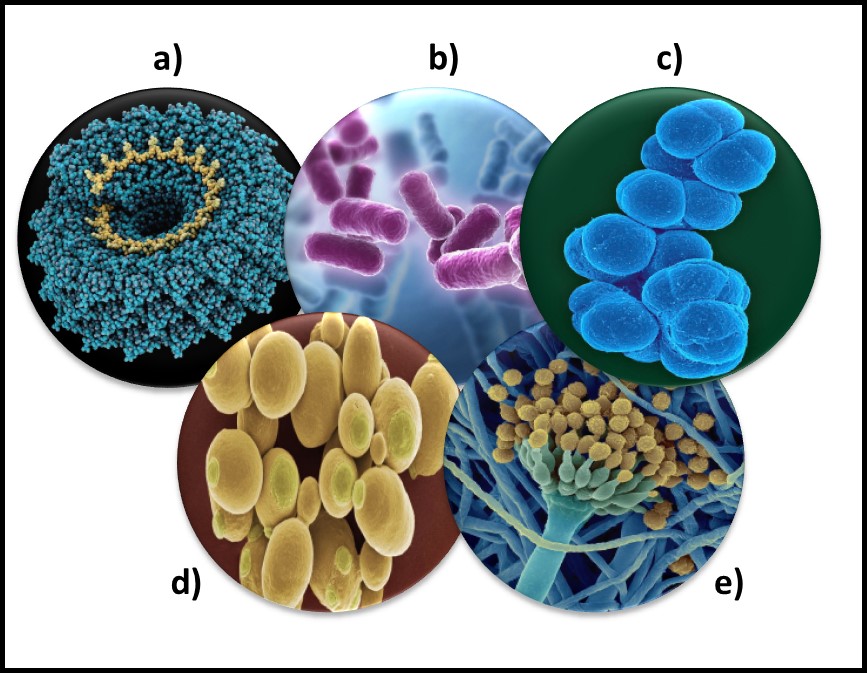
Microorganisms – a) virus; b) bacteria; c) archaea; d) yeast; d) mold.

Each year, on the first morning of STLE’s Metalworking Fluid Management Certificate Training Course, I ask attendees about their backgrounds. Invariably, the majority have at least undergraduate degrees in chemistry, engineering, or chemical engineering. However, of the more than 600 people who have taken the course since 2004, fewer than 50 have had a microbiology course.

Globally, biodeterioration – damage that organisms cause – has been estimated to range between $100 billion and $500 billion annually. Of this, 70 % to 80 % of biodeterioration damage is caused by microorganisms. Add to this an estimated $1 trillion cost due to infectious disease. On the flipside, biotechnology is a $500 billion industry that is based on microbiology. Just considering the economic impact microbe have on our lives, one might reasonably ask why so few people have received the most rudimentary education about microbes. Perhaps it’s the six syllables in microorganism (mic-ro-org-an-is-m) and microbiology that make the topic so intimidating. Still, given the role of microbes in disease, nature’s primary cycles, and biotechnology, one might think that every high school graduate would have learned something about microbiology. In this post and the next several to follow, I will do my best to demystify microbiology.

In this month’s article and those that follow, I’ll offer a very superficial overview of microbiology from an ecological and industrial perspective. There are numerous, excellent introductory microbiology textbooks. I don’t intend to provide any level of detail approaching that of a microbiology textbook. My intention is to help non-technical readers gain a fundamental appreciation for how microbes can affect their lives and their businesses.

Definition

Microorganisms (micro – meaning: small + organism – meaning: something having many related parts that function together as a whole) are living things that are too small to be seen by the naked eye. Microbiologists agree that bacteria, archaea, and some fungi (yeasts and molds) are microorganisms.

The status of virus is still a matter of debate. Viruses are essentially genetic material packaged in a protein coat. They don’t perform most of the functions that are used to define living beings. Thus most microbiologists do not consider viruses to be life forms. However, viruses reproduce by infecting cells and hijacking their victim’s (host’s) metabolic machinery to reproduce. Consequently, some microbiologists believe viruses should be classified as living things. Image (a) in the title figure shows a tobacco mosaic virus (TMV). The TMV virus is structurally complex, regardless of how we classify it. I included a virus in the in the figure because there are research groups investigating the use of viruses to control microbial contamination in industrial systems. I’ll return to this topic in a future post.

Abundance

One recent study, illustrated in Figure 1, estimated that microorganisms represent ~17% of Earth’s total biomass (estimated total biomass 550 gigatons of carbon – Gt C; 1Gt = 10⁹ tons – and bacterial biomass ≈70 Gt)¹. The contribution of bacteria to the Earth’s biomass is second only to that of plants. Microorganism biomass – including that of archaea, bacteria, fungi, protists, and viruses – account for ~93Gt.

A microbiome is the population of all microbes living in a specific ecosystem (fuel tank, cooling tower, human gut, etc.). Researchers investigating the human microbiome have estimated that the average human body has between 1x to 10x as many microbial cells as human cells. Moreover, it has been discovered that tissues, long thought to be microbe-free, have specific microbiomes that are likely to be essential for healthy tissue function (we have known about skin and gut microbes for nearly 170 years, but finding microbiomes specific to nearly every human tissue type (organs, muscle, etc.) was a surprise. Investigators have only scratched the surface of human microbiome research. We have little idea of how microbes interact with human cells and what roles they play in maintaining good health.

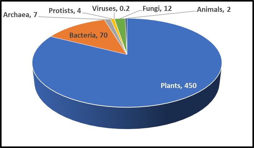
Fig 1. Relative abundance of Earth’s lifeforms, in Gt.

Diversity

As I will explain in future articles, the microbial world is remarkably diverse. The number of different types of bacteria has been estimated to range from hundreds of thousands to tens of millions, of which only a fraction of a percent has been identified.

I’ll discuss why below. Despite their central importance to life as we know it, even the most rudimentary discussion of microorganisms or microbiology (i.e., the study of microorganisms) is rarely included in high school or university curricula.

A Brief History

Tree of Life

Microbes were the first organisms to exist on earth. Our current understanding is that Earth formed 4.6 billion (4,600,000,000) years ago. There is evidence that the first microbes came into existence approximately 3.5 to 3.8 billion years ago (the fossil record indicates that mammals appeared 65 million years ago, and humans showed up a mere 315,000 years ago). Figure 3 illustrates the life on Earth timeline. The bar illustrating Earth’s age is 5 inches (in) long and the one for microorganisms is 4.1 in long. By comparison, the one for plants is 0.2 in and the one for humans is 0.000003 in – too thin to see! Thus, for more than 3 billion years, microbes were the only life forms on Earth.

If we visualize life as a tree, the organisms began to diversify genetically approximately 3.2 to 3.5 billion years ago (Figure 3). This was the time of the last universal common ancestor – LUCA – of all cellular organisms, starting with the bacteria and (thus far) culminating in humans. Before the microbes now classified as members of the kingdom Archaea were discovered near ocean floor, thermal vents in the Marianas Trench, in 1960, the tree of life was thought to have three Kingdoms: Monera (Prokaryota – all single cell organisms that do not have a nucleus or other membrane-bound internal bodies, Protista – all single cell organisms with a nucleus and other membrane-bound bodies, and Eukaryota – all multicellular organisms). As depicted in Figure 3a, in the 1960s through 1990s, Archaea were classified as Archaebacteria. When viewed through a microscope, they appeared to be bacteria. Believing that conditions around Marianas Trench thermal vents was similar to those of primordial Earth, microbiologists initially assumed that Archaea were more ancient than true bacteria – Eubacteriales. As genetic tools became available in the early 1990s, it became apparent that a) Eubacteriales are more ancient than Archaea (Figure 3b), and b) the Archaea are sufficiently distinct genetically to be its own phylogenic Kingdom (phylogenics – the study of evolutionary development and diversification of a species or group of organisms). When Figure 3a was created, fungi were thought to be much more ancient than plants or animals. As Figure 3b illustrates, the phylogenetic tree of life branched off to fungi, plants, and animals a mere half-billion years ago. Thus, fungi are more closely related to us than they are to bacteria.

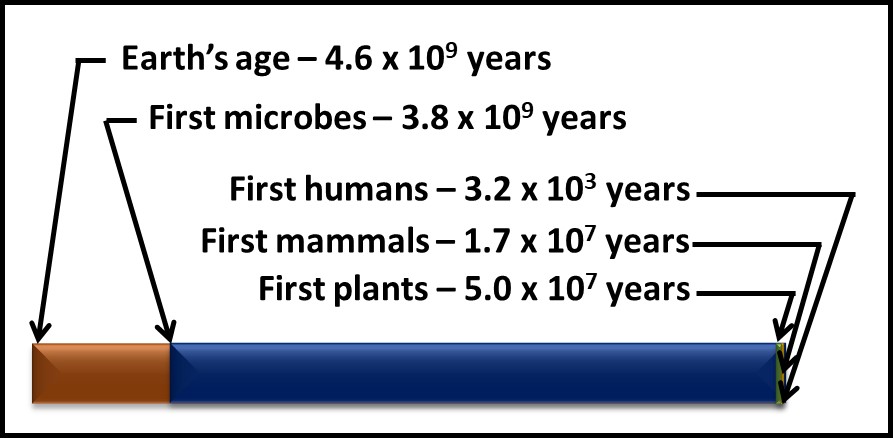
Fig 2. Timelines – microorganisms appeared approximately 1 billion years after Earth was formed and more than 3 billion years before the first plants appeared. Brown bar – Earth’s age; blue bar microorganisms’ age; green bar – time since plants first appeared; yellow bar – time since first animals appeared; purple bar (invisibly narrow line) – time since humans appeared.

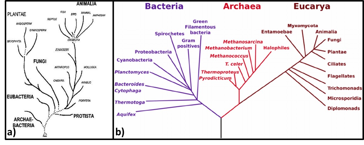
Fig 3. Phylogenic trees – a) Tree from mid-1960s depicting Archaebacteria as being more ancient than Eubacteria; b) Woese et al. (1990²) phylogenic tree showing three Kingdoms – Bacteria, Archaea, and Eucarya. Line segment lengths are based on genetic differences (longer lines indicate greater differences). The initial split at bottom center is LUCA.

Genomic testing has been a cottage industry since the late 1990s. A recent diagram (Figure 4) is based on the genomics of 2.3 million different species, from bacteria to humans, illustrates how complex the Tree has become (or as some authors note, the Tree now looks more like a Bush).

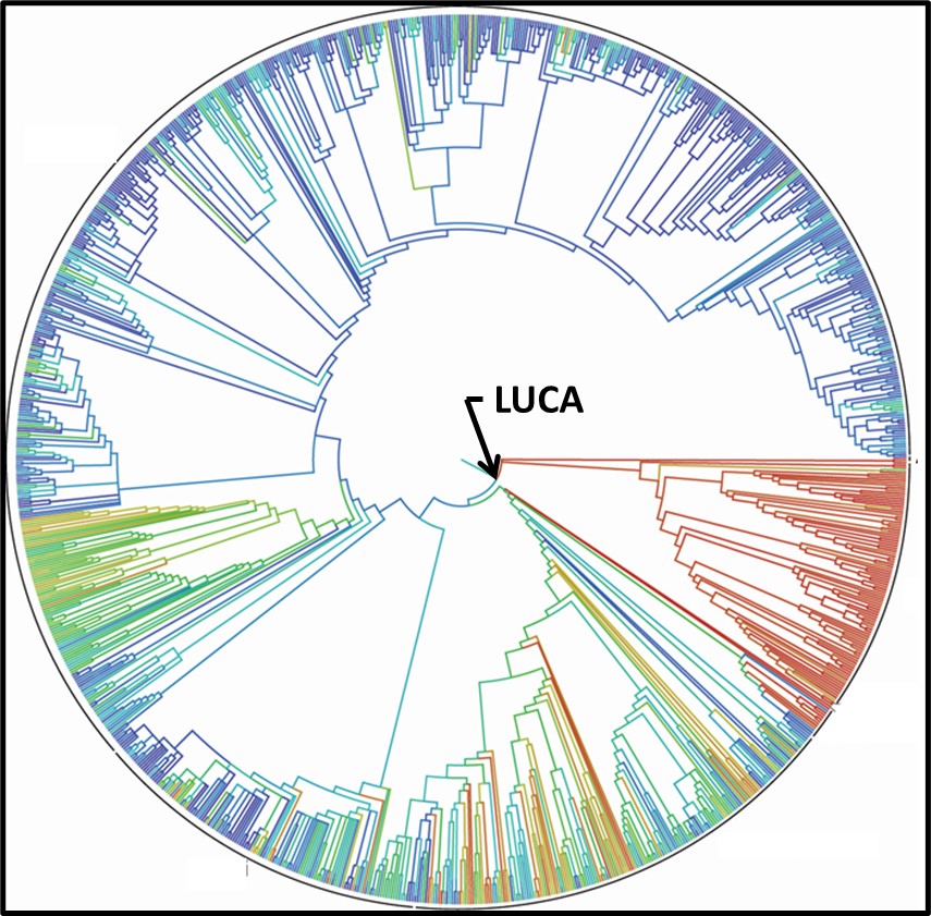
Fig 4. 2015 Tree of Life based on genetic data from 2.3 species.³

Human Awareness

Humans have been using microbes from time immemorial. We have been fermenting grains and grapes, and making cheeses, for as long as we have been cultivating plants or maintaining livestock. Modern microbiology dates from 1665, when Roert Hooke published Micrographia: or some Physiological Descriptions of Minute Bodies made by Magnifying Glasses with Observations and Inquiries Thereupon. A decade later, Antonie van Leeuwenhoek published his observations. Hooke and van Leeuwenhoek had each constructed microscopes through which they observed and created sketches of microorganisms (Figures 5a and 5b). However, it took another 200 years before Louis Pasteur and Robert Koch demonstrated that microbes were living beings and were responsible for fermentation, disease, and spoilage.

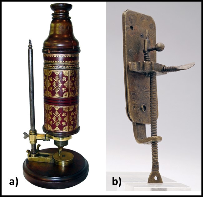
Fig 5. First microscopes – a) replica of Robert Hook’s microscope; b) replica of Antonie van Leeuwenhoek’s microscope.

Louis Pasteur conducted experiments to disprove the theory of spontaneous generation (belief that microbes developed from inanimate components of the materials which they caused to rot) and prove the germ theory of disease (i.e., that microorganisms did not form spontaneously and that they caused disease, biodeterioration, and were the agents responsible for fermentation). Pasture used goosenecked flasks (Figure 6) to demonstrate that microbes did not proliferate (multiply) in broth boiled in the flasks but did in identical flasks that contained unboiled broth. Proliferation also occurred when Pasteur intentionally permitted boiled broth to be exposed to microbially contaminated air (i.e., either by breaking off the gooseneck or tipping the flask). The gooseneck shape allowed air but not microbes to enter the flasks. These experiments led to Pasteur’s development of the pasteurization – the process of heating substances at temperatures sufficient to disinfect but not degrade them.

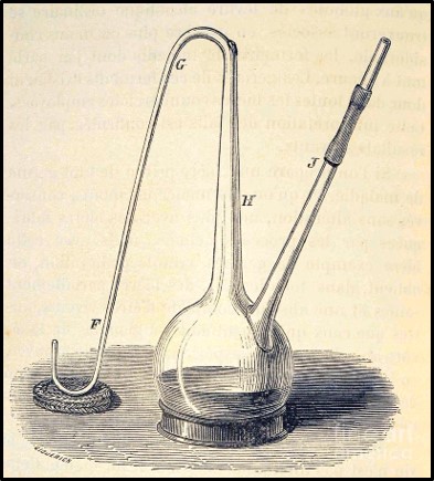
Fig 6. Drawing of Louis Pasteur’s gooseneck flask used to disprove spontaneous generation theory.

While Pasteur was focusing on fermentation microbiology, Robert Koch demonstrated the unequivocal relationship between microbes and disease. Koch demonstrated that the disease, anthrax was caused by the spore forming bacterium, Bacillus anthracis. He also developed the first solid growth media so that he could isolate pure cultures from colonies (Figure 7, zone 5). Pasteur’s and Koch’s research launched the modern age of microbiological research.

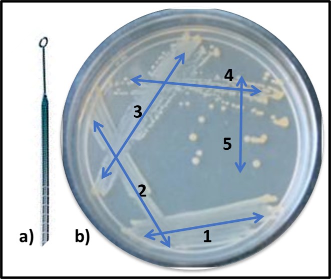
Fig 7. Obtaining a pure (single type of bacterium) culture by the streak plate method – a) specimen is collected using a sterilized inoculating loop; b) successively, initial specimen is deposited onto solid nutrient medium using a back-and forth motion (1), inoculating loop is heat sterilized, cooled, and oved across initial inoculation zone (2). This dilutes the sample. The final iteration (5) typically produces individual colonies after the inoculated plate has been incubated.

As now, much of the research performed during the late 19th century was focused on the relationship between microbes and disease. However, Sergei Winogradsky became the father of microbial ecology. Based on his pioneering research on sulfur metabolism in the late 1880s, Winogradsky developed the theory of biogeochemical cycles. This theory states that elements like sulfur, carbon, nitrogen, and phosphorous cycle through nature (Figure 8). These cycles are primarily mediated by microbial activity. The first paper describing gasoline deterioration by microbes was published in 1895. Starting in the 1920s, considerable effort was focused on oilfield damage caused by microorganisms. This research included the first studies on what was originally called microbially induced corrosion (MIC – now microbiologically influenced corrosion – see MICROBIOLOGICALLY INFLUENCED CORROSION – Biodeterioration Control Associations, Inc. (biodeterioration-control.com)). However, the term biodeterioration was not coined until 1965, when H. J. Hueck offered the definition: “any undesirable change in the properties of a material caused by the vital activities of organisms.”⁴

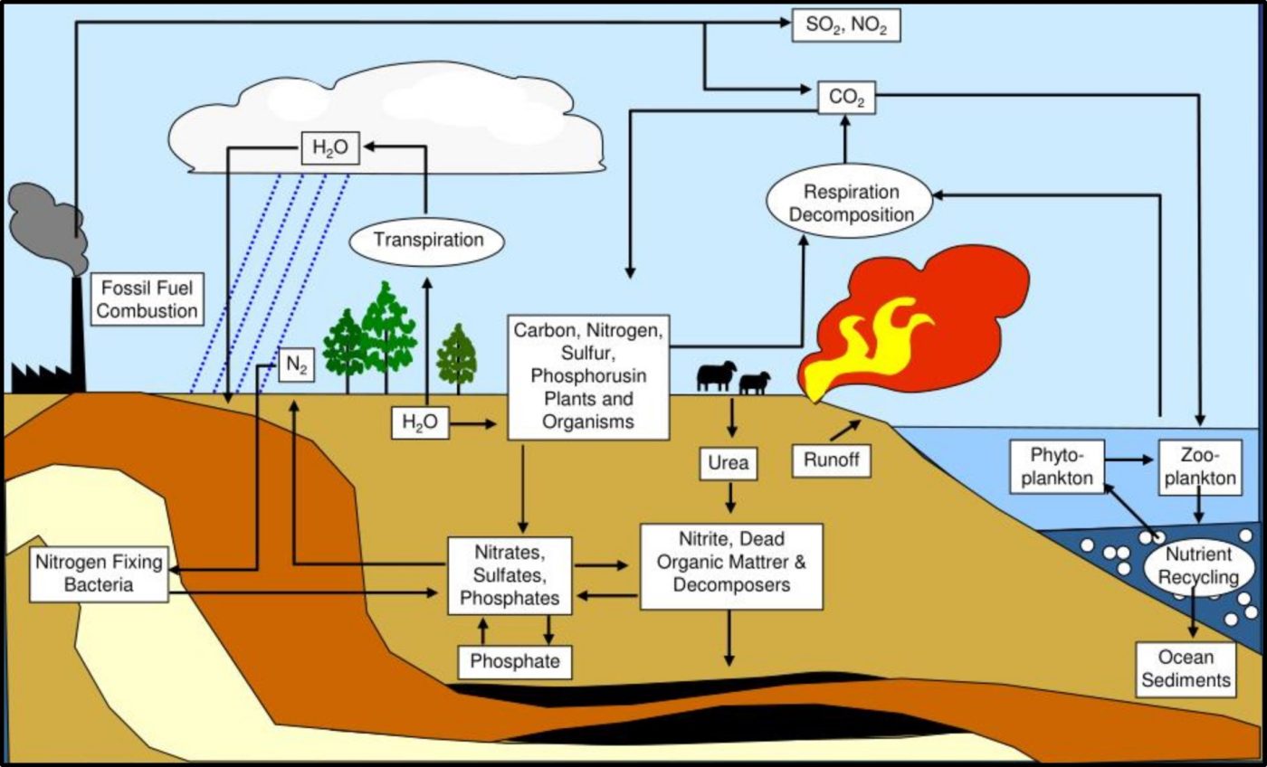
Fig 8. Biogeochemical cycles – this illustration provided a simplified depiction of how carbon (C), nitrogen (N), phosphorous (P), and sulfur (S) cycle through nature.

In my seminars on the topic I explain that biodeterioration and bioremediation are two sides of the same biodegradation coin (Figure 9). As Winogradsky observed, microbes drive biogeochemical cycles. These cycles occur regardless of human intent. When we want biodegradation to occur, we call it bioremediation. When microbial activity causes changes, we’d prefer to prevent, we call it biodeterioration (see https://biodeterioration-control.com/2018/03/).

Fig 9. Like the obverse (front) and reverse (back) sides of this 2000 Sacagawea U.S. dollar coin, bioremediation and biodeterioration are flips sides of biodegradation.

Summary

Microbes play invaluable roles in our lives. Our bodies would not function without the microbes that make up he human microbiome. Fewer than 2,000 pathogenic microbes have been identified among the tens of thousands that have been identified and the millions of different types of microbes that exist in nature. Microbes mediate nutrient cycles. This cycling conserves essential nutrients and prevents wastes from accumulating. Biodegradation includes all processes that breakdown organic substances. On one hand, biodegradation is the foundational element of a $0.5 trillion biotechnology industry. On the other, biodeterioration and infectious disease cost $1.5 trillion per year. We are part of the microbial world. To me, that seems like an excellent reason why everyone should have a basic understanding of microbiology.

For more information about fuel system condition monitoring and predictive maintenance, contact me at fredp@biodeterioration-control.com.

¹ Bar-On, Y.M, Phillips, R., Milo, R., 2018. The biomass distribution on Earth. Proc Natl Acad Sci U S A., 115(25):6506-6511. https://pubmed.ncbi.nlm.nih.gov/29784790/.
² Woese, C. R., Kandler, O., Wheelis M.L., 1990. Towards a natural system of organisms: proposal for the domains Archaea, Bacteria, and Eucarya. Proceedings of the National Academy of Sciences of the United States of America. 87 (12): 4576–9. https://doi.org/10.1073/pnas.87.12.4576.
³ Hinchliff, C. et al., 2015. Synthesis of Phylogeny and Taxonomy Into a Comprehensive Tree of Life. Proceedings of the National Academy of Sciences https://www.pnas.org/doi/full/10.1073/pnas.1423041112.
⁴ Hueck, H.J., 1965. The Biodeterioration of Materials as a Part of Hylobiology. Material und Organismen, 1, 5-34.

BIODETERIORATION ROOT CAUSE ANALYSIS – PART 4: CLOSING THE KNOWLEDGE GAPS

Refresher

In my March 2021 article, I began a discussion of root cause analysis (RCA). In that article I reviewed the importance of defining the problem clearly, precisely, and accurately; and using brainstorming tools to identify cause and effect networks or paths. Starting with my April 2021 article I used a case study to illustrate the basic RCA process steps. That post focused on defining current knowledge and defining knowledge gaps. Last month, I covered the next two steps: closing knowledge gaps and developing a failure model. In this post I’ll complete my RCA discussion – covering model testing and what to do afterwards (Figure 1).

Fig 1. Common elements shared by effective RCA processes.

Step 7 Test the Model

As I indicated at the end of May’s post , the data and other information that we collected during the RCA effort led to a hypothesis that dispenser slow-flow was caused by rust-particle accumulation on leak detector screens and that the particles detected on leak detector screens were primarily being delivered with the fuel (regular unleaded gasoline – RUL) supplied to the affected underground storage tanks (UST).

Commonly, during RCA efforts both actionable and non-actionable factors are discovered. An actionable factor is one over which a stakeholder has control. Conversely, a non-actionable factor is one over which a stakeholder does not have control. Within the fuel distribution channel, stakeholders at each stage have responsibility for and control of some factors but must rely on stakeholders either upstream or downstream for others.

For example, refiners are responsible for ensuring that products meet specifications as they leave the refinery tank farm (Figure 2a – whatever is needed to ensue product quality inside the refinery gate is actionable by refinery operators), they have little control over what happens to product once it is delivered to the pipeline (thus practices that ensure product quality after it leaves the refinery are non-actionable).

Pipeline operators (Figure 2b) are responsible for maintaining the lines through which product is transported and ensuring that products arrive at their intended destinations in the – typically distribution terminals in the U.S. – but are limited in what they can add to the product to protect it during transport.

Terminal operators can test incoming product to ensure it meets specifications before it is directed to designated tanks. They are also responsible for maintaining their tanks so that product integrity is preserved while it is at the terminal and remains in-specification at the rack (Figure 2c). Terminal and transport truck operators have a shared responsibility that product is in-specification when it is delivered to truck tank compartments (solid zone where Figures 2c and 2d overlap).

Tanker truck operators are also responsible for ensuring that tank compartments are clean (free of water, particulates, and residual product from previous loads). Additionally, truck operators (Figure 2d) are responsible for ensuring that tanker compartments are filled with the correct product and that correct product is delivered into retail and fleet operator tanks. They do not have any other control over product quality.

Finally, retail and fleet fueling site operators are responsible for the maintenance of their site, tanks, and dispensing equipment (Figure 2e).

Regarding dispenser slow-flow issues, typically only factors inside the retail sites’ property lines are actionable (Figure 3 – copied from May’s post).

Fig 2. Limits of actionability at each stage of fuel product distribution system – a) refinery tank farm; b) pipeline; c) terminal tank farm; d) tanker truck; and e) retail or fleet fuel dispensing facility. Maroon shapes around photos reflect actionability limits at each stage of the system. Note that terminal and tanker truck operators share responsibility for ensuring that the correct, in-specification product is loaded into each tank compartment.

Fig 3. Dispenser slow-flow failure model.

As illustrated in Figure 3, the actions needed to prevent leak detector strainer fouling were not actionable by retail site operators. In this instance, we were fortunate in that the company whose retail sites were affected owned and operated the terminal that was supplying fuel to those sites.

A second RCA effort was undertaken to determine whether the rust particle issue at the retail sites was caused by actionable factors at the terminal. We determined that denitrifying bacteria were attacking the amine-carboxylate chemistry used as a transportation flow improver and corrosion inhibitor. This microbial activity:

– Created an ammonia odor emanating from the RLU gasoline bulk tanks,

– Increased the RUL gasoline’s acid number, and

– Made the RUL gasoline slightly corrosive.

Although the rust particle load in each delivery was negligible (i.e., <0.05 %), the total amount of rust delivered added up quickly. If the rust particle load was 0.025 %, 4 kg (8.8 lb) of particles would be delivered with each 26.5 m3 (7,000 gal; 19,850 kg) fuel drop. The sites received an average of two deliveries per week (some sites received one delivery per week and others received more than one delivery per day). That translates to an average of 32 kg (70 lb) of particulates per month. Corrective action at the terminal eliminated denitrification in the RUL gasoline bulk tanks and reduced particulate loads in the RUL gasoline to <0.01 %.

Step 8. Institutionalize Lessons Learned

Although the retail site operators could not control the quality of the RUL gasoline they received, there were several actionable measures they could adopt.

1. Supplemented automatic tank gauge readings with weekly manual testing, using tank gauge sticks and water-finding paste. At sites with UST access at both the fill and turbine ends, manual gauging was performed at both ends.

2. Use a bacon bomb, bottom sampler to collect UST bottom samples once per month. Run ASTM Method D4176 Free Water and Particulate Contamination in Distillate Fuels (Visual Inspection Procedures) to determine whether particles were accumulating on UST bottoms. As for manual gauging, at sites with UST access at both the fill and turbine ends, bottom sampling was performed at both ends.

3. Evaluate particulate load for presence of rust particles by immersing a magnetic stir bar retriever into the sample bottle and examining the particle load on the retriever’s bottom (Figure 4).

4. Set bottoms-water upper control limit (UCL) at 0.64 cm (0.25 in) and have bottoms-water vacuumed out when they reach the UCL.

5. Set rust particle load UCL at Figure 4 score level 4 and have UST fuel polished when scores ≥4 are observed.

6. Test flow-rates at each dispenser weekly – reporting flow rate and totalizer reading. Compute gallons dispensed since previous flow-rate test. Maintain a process control chart of flow-rate versus gallons dispensed.

Fig 4. Qualitative rust particle test – a) magnetic stir bar retriever; b) attribute scores for rust particle loads on retriever bottom, ranging from 1 (negligible) to 5 (heavy).

These six actions were institutionalized as standard operating procedure (SOP) at each of the region’s retail sites. Site managers received the requited supplies, training on proper performance of each test, and instruction on the required record keeping. There has been no recurrence of premature slow-flow issues at any of the retail sites originally experiencing the problem.

Wrap Up

Although I used a particular case study to illustrate the general principles of RCA, these principles can be applied whenever adverse symptoms are observed. I have used this approach to successfully address a broad range of issues across many different chemical process industries. The keys to successful RCA include carefully defining the symptoms and taking a global, open-minded, multi-disciplinary approach to defining the cause-effect paths that might be contributing to the observed symptoms. Once a well-conceived cause-effect map has been created, the task of assessing relative contributions of individual factors becomes fairly obvious, even when the amount of actual data might be limited.

Bottom line: effective RCA addresses contributing causes rather than focusing only on measures that only address symptoms temporarily. In the fuel dispenser case study, retail site operators initially assumed that slow-flow was due to dispenser filter plugging. Moreover, they never checked to confrim that replacing dispenser filters affected flow-rates. This short-sighted approach to problem solving is remarkably common across many industries. To learn more about BCA’s approach to RCA, please contact me at fredp@biodeterioration-control.com.

FUEL & FUEL SYSTEM MICROBIOLOGY PART 34 – Connecting the Dots, Part 2

Refresher from Part 1: What do Microbiology Test Results Mean?

In January’s Fuel & Fuel System Microbiology article I led with this question and commented that it is actually a double question. In one sense, it is asking: “Do my microbiology test results tell me conclusively whether microbes are damaging my fuel or fuel system?” In another sense, the question means: “Why don’t the results from different fuel microbiology test kits always agree?” I am then asked why often, even when microbiological test data indicate that there is heavy biocontamination present, the fuel does not seem to be affected. In today’s post – the second of three on this topic – I’ll discuss the relationship between microbiological test results and system damage.

Do My Microbiology Test Results Tell Me Conclusively Whether Microbes are Damaging My Fuel System?”

As I wrote, last month, the short answer is no. Keep in mind, all three of these posts about whether detected microbial contamination invariably signals biodeterioration is happening. This is different from the situation in which there are numerous indications of system biodeterioration, but microbiological test results are negative. I’ll revisit that issue in a future post.

Fuel System Biodeterioration

Biodeterioration is any damage caused by organisms. In fuel systems, the most common forms of biodeterioration are biofouling and microbiologically influence corrosion (MIC).

Biofouling is the result of microbes and the slime they produce (i.e., extracellular polymeric substance – EPS – the primary material in biofilms (see Part 15 for a refresher on biofilms) accumulating on system surfaces. When biomass accumulates on filters or screens, it restricts product flow. Figure 1 shows photographs of a dispenser filter, dispenser strainer, and leak detector strainer – each of which has become fouled with biomass.

Fig 1. Biofouling – a) dispenser filter; b) dispenser strainer; c) leak detector strainer.

Biofouling can also cause other problems including valves sticking or failing to close completely. When biofouling accumulates on the surface of an automatic tank gauge’s (ATG’s) water float (Figure 2a) the impact will depend on the biofilm. If the biofilm is filled with gas pockets, the float will be lighter than normal and will float within the fuel – giving a false signal that bottoms-water is present when it is not (Figure 2b). Conversely if the EPS is loaded with rust particles, the water float will be heavier than normal. It will rest on the tank bottom, even when 2 cm to 3 cm bottoms-water as accumulated (Figure 2c)

Fig 2. ATG water float – a) fouling on float’s surface; b) gas pockets in biofilm lift float into fuel-phase; c) rust particles in biofilm weigh-down float, preventing from floating above bottoms-water.

Biofilms coating vehicle fuel gauges will cause the gauges to give inaccurate readings.

Note that all of these biofilm accumulation zones are on system components. Fuel systems can have substantial bioburdens in tank bottom samples, but no biofouling. Although the possibility of fouling increases with increased bioburden in fuel tank bottom samples, detection of substantial microbial loads in fluid samples doesn’t necessarily mean that fouling has occurred. The only way to know for certain whether biofouling has occurred is by direct inspection of the fuel system components that are likely to become fouled.

Microbiologically influenced corrosion (MIC) includes any from of material damage that is caused either directly or indirectly by microbes. Most commonly, MIC is related to metallic components, but polymeric materials are also susceptible to MIC.

Contamination Detection

Connie Francis recorded Where the Boys Are as the title track for the 1961 movie of the same name. The next several paragraphs could be titled Where the Microbes Are. Microbial contamination is not a fuel property. Unlike fuel properties, the distribution of microbes in fuel systems is non-uniform (heterogeneous). The heterogeneous distribution of microbial contamination makes it difficult to collect a sample that is guaranteed to contain microbes – even if microbial contamination is present in the fuel system.

In my fuel microbiology courses I recount a lecture I heard as an undergraduate. My professor was part of the team tasked with developing a reliable test method for determining whether there was life on Mars. One member of the team suggested using a camera that would scan the horizon for signs of life. The device would scan 15 ° of arc at a time, completing a 360 ° scan each hour. The counterargument – illustrated in figure 3 – was that large life forms (elephants in figure 3) might be present but missed entirely because they continually moved out of the camera’s line of sight.

Fig 3. Not detecting the elephants – a) elephants are to the east while camera is pointing west; b) elephants are to the west while camera is pointing east. A researcher viewing the camera’s photo record would conclude that there are no elephants in the area photographed!

Now consider a 0.5 L (0.13 gal) sample collected from the bottom of a 38,000 (38 m3, 10,000 gal) tank. The sample represents 0.001 % of the total liquid volume in the tank. Similarly, a bottom sample from the bottom of a tank with a 31 m2 (31,000 cm2, 334 ft2) surface area draws in fluid, sludge, and sediment form a 3 cm to 5 cm radius. That represents 0.02 % of the total bottom surface area. Figure 4 illustrates how a two bottoms samples, taken from spots just a few cm apart, can have substantially different bioburdens.

Fig 4. UST bottom – biomass density heat map. Green zones have negligible biomass accumulation. Red zones have > 5 mm thick masses. Numbered blue circles are points from which bottom samples were collected. Distance between #1 and #3 ≈ 0.25 m (10 in). Microbial loads: #1 – below detection limits; #2 – moderate bioburden; #3 – heavy bioburden.This is why I argue that a sample that yields negative microbiological test results provides much less information than one that yields positive results. You can get negative test results from samples taken in tanks suffering from severe biodeterioration damage. The converse is also true: it’s possible to detect substantial bioburdens in systems that show no indication of biodeterioration. In the latter case, the microbiology data triggers further checks. The cost of performing these checks is a fraction of the cost of post-failure corrective maintenance (i.e., tank replacement, site remediation, etc.).

Bottom Line

Fuel system samples used for microbiological testing are meant to be diagnostic – not representative. To be reliably diagnostic, samples must come from locations most likely to harbor microbes. This is can be impractical (if not impossible). Consequently, samples from systems with substantial fouling, MIC, or both can have negligible detectable bioburdens. Conversely, it is not uncommon for systems from which samples have apparently heavy bioburdens to have no biodeterioration symptoms. In Connecting the Dots – Part 3, I’ll write about why test results from different microbiology methods can lead to different conclusions. As I was writing today’s blog I decided to add a Part 4 – the impact of specific microbial activities on the link between bioburden and biodeterioration.

The details

For more details about understanding the relationship between microbiology test data and fuel or fuel system biodeterioration, please contact me at either fredp@biodeterioration.control.com or 01 609.306.5250.

FUEL & FUEL SYSTEM MICROBIOLOGY PART 31 – MATCHING THE SAMPLING TOOL WITH THE SAMPLING OBJECTIVE

Dixon Pumps Fuel System Broadcast Emails

The folks at Dixon Pumps dixon@dixonpumps.com routinely send out broadcast emails about fuel system maintenance. Today’s article was inspired by their 31 October 2019 email: Water Removal Basics, by Patrick Eakins. After the fourth paragraph, Mr. Eakins has an action list. The first action he recommends is:

“1. Determine the volume of phase (e.g. free water, ethanol) at the bottom of the tank. This can be accomplished by using a fuel sampler. First take a sample on the very bottom of the tank, then at 1-inch increments until you determine where the phase ends and the fuel begins.”

The phrase: “using a fuel sampler” caught my attention and will be this article’s focus. Spoiler alert: In Fuel Microbiology Part 30, I wrote about fuel system sampling. In this article be covering some – but not all – of the same material.

What Sampler?

The Dixon Pump article advises folks to use a sample but makes no mention of what kind of sampler is best for determining the height of free-water (or phase-separated ethanol and water) in underground storage tanks. The problem with an open statement like this is that the samples obtained by different types of samplers tell different stories.

Bacon Bomb Samplers

The Bacon bomb is probably the best, currently available bottom sample. Part 30, figure 2a shows a photo of a chrome-plated Bacon Bomb sampler. Figure 1, is a photo of a Bacon Bomb with a clear, polymeric cylinder (the cylinder is the sampler’s primary container). To make it easier to clean, the cylinder is threaded at each end so that the cap and bottom can be removed. The cap and plunger each have a hole for inserting a ring clip. To facilitate lowering and retrieving the sampler into tanks, a sounding tape can be attached to the cap’s ring. A secondary line can be attached to the piston’s ring for sampling above the tank’s floor (when the sampler is at the desired depth, the secondary line is pulled for approximately 30 sec to allow the sampler to fill. It is then released so that the piston is sealed against the sampler’s inlet).

Fig 1. Bacon Bomb sampler.

Figure 2 illustrates what happens when a Bacon Bomb sampler is used to collect a bottom sampler. The piston rests against the sampler’s inlet as it is lowered through the fuel column (figure 2a1 and 2b1). When the piston contacts the tank bottom, it is pushed up to open the inlet (figure 2a2 and 2b2). Hydrostatic pressure from the fuel column forces fluid into the sampler. When the Bacon Bomb is lifted off of the tank bottom, the piston will drop back into place – sealing it closed with the sample retained inside the cylinder. If there is no water or sludge present, the sampler will fill with fuel (figure 2a3). However, if bottoms-water is present, it will be the first fluid to enter the sampler. Thus, if there was 500 mL or water, and the Bacon Bomb’s capacity was 500 mL, the sample would be all, or nearly all water (figure 2b3). This would not be an accurate means for estimating the tank’s water level.

Fig 2. Bottom sample collection using a Bacon Bomb sampler. a) No water on tank bottom: 1) as sampler is lowered through fuel, the piston’s seat rests against the sampler bottom’s inlet, preventing fluid from entering; 2) when the piston touches the tank bottom and sample continues to fall, the inlet is opened and fluid enters – driven by the force of the fuel column’s hydrostatic pressure; 3) as the sampler is lifted off the tank bottom, the piston once again falls to reseal the sampler’s inlet – retaining the sampled fluid. b) Bottoms-water present: 1) same as a1; 2) any bottoms-water and sediment are pushed into sampler before any overlying fuel can enter; 3) same as a3, but now sampler is filled with water instead of fuel.

What does this mean in practical terms? Take a look at figure 3. Three, 500 mL Boston round bottles were filled from Bacon bomb samples collected from a tank bottom. The first sample (figure 3a) captured 450 mL bottoms-water and 50 mL of diesel fuel. If this had been used to estimate the water level, one might have concluded that the tank bottom was covered with a 5 in (13 cm) high water-layer. All 490mL of 500 mL from the second Bacon bomb sample (figure 3b) was bottoms-water. Was there actually 6.7 in (17 cm) of bottoms-water? The third sample (figure 3c) was mostly fuel. Three successive Bacon bomb samples from the same spot were sufficient to pull most of the water out of the tank. Water paste had shown that at the fill-end, the tank had 0.5 in (1.2 cm) of water.

Fig 3. Three successive Bacon bomb samples form one sampling point. A, b, and c were the fist, second, and third samples, respectively.

Bailer Samplers

Bailer samples are normally used to collect fluids from monitoring wells. Figure 4a illustrates how monitoring wells are placed around underground storage tanks. Note that the bottom of the well is porous and at a depth below the water table. After sample collection, the contents of the bailer sampler are layered – reflecting the layering of fuel over ground water in the well (figure 4b – normally the sampler will contain only water). Figure 4c shows the primary components of a bailer sampler. There are numerous bailer designs. For sampling fuel tank bottoms, the sampler must be fabricated form fuel-compatible materials. Also, as shown in figure 4c, the bailer should have a flat bottom.

Fig 4. Monitoring wells and bailer samplers. a) schematic showing location of a monitoring well near a UST; b) bailer sampler retrieved from monitoring well – dark fluid next to ruler is leaked fuel that was captured in monitoring well; c) bailer sampler showing its key parts.

To collect bottom samples, the bailer is slowly lowered through the fuel column (figure 5a1 and 5b1) until it stands vertically on the tank floor (figure 5a2 and 5b2). Because it is not sealed as it descends through the fluid, it analogous to collecting a soil core sample (figure 6). Most bailer samplers have a ball that floats inside the cylinder as the sample is lowered, then settles to the base and seals the inlet as the sampler is raised (figure 5a3 and 5b3). As shown in figure 5c, just as with a soil core sample, the bailer sample reflects the profile of water, rag layer, and bottom fuel much as they are layered in the tank’s bottom. There is typically ∼0.25 in (∼1 cm) between the bailer’s bottom and the inlet. Consequently, bailer samplers are not good for collecting bottom sludge and sediment samples. However, they are useful for estimating bottoms-water height. The tank from which the figure 5c sample was taken had ∼3.5 in (∼9 cm) bottoms-water and 0.75 in (1.9 cm) thick rag layer. The water height in the sampler agreed well with that determined using water paste.

Fig 5. Bottom sample collection using a bailer sampler. a) No water on tank bottom: 1) as sampler is lowered through fuel, ball floats above sampler inlet; 2) when sampler comes to rest on tank bottom, the ball sinks to the inlet; 3) as the sampler is lifted off the tank bottom, the ball seals the sampler’s inlet – retaining the sampled fluid. b) Bottoms-water present: 1) same as a1; 2) water fills the sample to the level of bottoms-water in the tank; 3) same as a3, but now sampler has fuel over water; c) fuel tank bailer sample.

Fig 6. Soil core sampler. a) core sampler pressed into soil; b) soil core, showing three soil horizons: a – organic surface zone, b – surface soil, and c – subsoil.

Other Samplers

ASTM Practice D4057 describes other fuel samplers. However, none of these are useful for collecting true bottom samples.

Best Practice for Determining Height of Bottoms-Water Layer

As I explained in my previous fuel microbiology post, the best way to determine bottoms-water height is by coating either a sounding sick or bob with water paste and lowering it into the tank. The water will react with the paste to change its color. Because tanks are rarely level, best practice is to test for water at two – preferably three- points: fill end, ATG (automatic tank gauge well, and fill end).

The details

For more details about fuel tank bottom sampling and water accumulation determination, please contact me at either fredp@biodeterioration.control.com or 01 609.306.5250.

FUEL & FUEL SYSTEM MICROBIOLOGY PART 29

What Does “Viable But Not Culturable” Mean and Why Should I Care?

In microbiology, the term used to describe microbes that appear to be healthy and active by test methods other than culturing is viable but not culturable – VNBC. Since the term first came into vogue in the 1980s, it has always reminded me of the Monty Python skit in which the customer – played by John Cleese – and the shop owner – played by Michael Palin – debate whether the parrot that Mr. Cleese had just bought was dead or simply resting, check it out at The Parrot Sketch.

Michael Palin (left) and John Cleese (right) in Monty Python’s “Pet Shop Sketch” (1969).

The viability versus culturability debate

The issue is relevant for two reasons. First, if a fuel or other industrial process fluid system (think heat exchange fluids, metalworking fluids, lubricating oils and hydraulic fluids) is home to a population of microbes that are biodeteriogenic (i.e., causing damage to the fluid, the system, or both) but are not detected by culture testing, the risk of experiencing a failure event can high.

Second, the term VNBC has numerous meanings – depending on researchers’ focus. The varied definitions creates confusion among both microbiologists and others who rely on microbiological test results to drive maintenance decisions.

What does viable mean?

The Online Biology Dictionary defines viable as an adjective meaning (“1) Alive; capable of living, developing, or reproducing, as in a viable cell.” ASTM is a bit more helpful offering several similar definitions. From F2739 Guide for Quantifying Cell Viability within Biomaterial Scaffolds we get: “viable cell, n – a cell capable of metabolic activity that is structurally intact with a functioning cell membrane.” D7463 and E2694 offer: “viable microbial biomass, n – metabolically active (living) microorganisms.” These slight variations all agree that viability relates to a microbe’s ability to:

function under favorable physical and chemical conditions (more on this in a bit), or
to survive in an inactive (dormant) state under unfavorable conditions, and
to become active again once conditions improve.

What does culturable mean?

ASTM defines culturable as an adjective: “microorganisms that proliferate as indicated by the formation of colonies on solid growth media or the development of turbidity in liquid growth media under specific growth conditions.” This definition is used in several ASTM standard test methods, guides, and practices.
When microbes reproduce – i.e., proliferate – go through repeated cycles of division – on a solid or semi-solid medium, after approximately 30 generations (doubling cycles, or generations) they accumulate enough mass to form a visible colony. Thirty generations (230) yields approximately a billion cells. Liquid growth media become visibly turbid once the population density (cells mL-1) reaches approximately one million (106) cells – 20 generations. The duration of a single generation varies among microbial species and growth conditions. At present, known generation times range from 15 min for the fastest proliferating bacteria to >30 days (recent discoveries of deep earth microbes suggest that these microbes might have generation times measured in years or decades – the generation time for humans is approximately 30 years). The key point is that culturable, microbes reproduce in or on growth media under specific environmental conditions.

Before leaving our discussion of culturable lets consider time. Microbes with 15 min generation times will turn broth media turbid in 5h to 6h and form visible colonies on solid media within 8h to 10h. For microbes with a 1h generation time, detection as turbidity or colonies lengthens to 20h and 30h respectively. Many culture-based test protocols state that final observations are to be made after 3-days – sometimes 5-days. Any microbe with a generation time longer than 4h is unlikely to produce a visible colony within 5-days. They will not be detected unless observations are continued for a week or longer. For example, the culture test for sulfate reducing bacterial is not scored negative until after 30-days observation. If you end a culture test at 3-days, are all of the slower growing microbes non-culturable?

What are growth media?

Since the mid-1850s, microbiologists have developed thousands of different recipes designed to support microbial growth and proliferation (recall from an early post that growth refers to the increase in mass, and as noted above, proliferation refers to an increase in numbers). Some growth media are undefined. They are simple recipes made up of extracts from yeasts, soy, and animals. These are the components of media used for the most common culture test: the standard plate count. Other media are prepared from individual chemicals. Their recipes can include more than a dozen ingredients. Solid and semi-solid media include a gelling agent such as agar (extracted from seaweed), gelatin, or silica gel. One of the most frequently referenced microbiological media cookbooks – the Difco Manual – lists more than a thousand recipes. Each of these recipes was developed to detect one or more types of microbes. In addition to the diversity of recipe ingredients, growth media vary in pH, total nutrient concentration (some microbes cannot tolerate more than trace concentrations of nutrients), and salts concentration (ranging from deionized water to brine). The microbes targeted for recovery dictate post-inoculation incubation conditions. Some microbes require an oxygen-free (anoxic) environment. Others require special gas mixtures. Microbes also vary widely on the temperatures at which they will grow. Some only grow at temperatures close to freezing. Others require temperatures closer to boiling.

The growth medium defines the chemical environment and the incubation conditions define the physical environment in which microbes are cultured. No single growth medium is likely to support the proliferation of more than a tiny fraction of the different types of microbes present in an environmental sample. Many microbiologists estimate that <0.1 % of the microbes in a sample will be culturable in a given medium. Similarly, we suspect that for every microbe that has been cultured, there are at least a billion that haven’t.

Is my microbe really dead or simply resting? When conditions are unfavorable to either growth, proliferation or both, many different types of microbes have coping mechanisms. For nearly 200 years, we have recognized that some types of microbes can form endospores – their cell wall chemistry changes and metabolic activity ceases. Only in the past 20 years, we have come to recognize that non-spore-forming microbes can enter into a dormant state that enables them to survive unfavorable conditions for centuries or millennia – becoming metabolically active once conditions once again become favorable. Moreover, in some environments, although the microbes are metabolically active, the rate of their activity is so slow as to be nearly undetectable.

Within some fields of microbiology, VNBC refers to microbes that have been injured due to exposure to a microbicide. Pre-incubation in so-called recovery media – improves their ability to reproduce in or on growth media. In my opinion, this is a very myopic view of VNBC.

Microbial ecologists define VNBC as microbes that are metabolically active or dormant in their home environments but will not growth on the culture media and incubation conditions used to detect them.

I first experienced this phenomenon in the 1970s when I was testing water from oilfield production wells. Using radioactive carbon labelled nutrients to measure metabolic activity, my team routinely found that samples that yielded <1 CFU mL-1 (CFU – colony forming unit: “a viable microorganism or aggregate of viable microorganisms, which proliferate(s) in a culture medium to produce a viable colony.” ASTM E2896) held very active populations. Poisoned controls demonstrated that conversion from radiolabeled acetic acid or glucose to radiolabeled carbon dioxide was from metabolic activity – not from a non-biological (abiotic) process.

This means that culture testing invariably underestimates the microbial population density in tested samples. Conversely, because microbes that were dormant in the environment from which they were sampled can become active once transferred into or onto nutrient media, culture testing can overestimate the presence of metabolically cells. For example, most microbes suspended in fuels or lubricants are dormant, but can become active and form colonies on growth media. These issues do not make culture testing good or bad. Culture testing is still the only practical tool for obtaining microbial isolates that can be used for further testing. Moreover, culture testing is a useful condition monitoring tool if you are tracking changes over time. The more important limitation of culture testing as a condition monitoring tool is the delay between test initiation and the availability of test results. In the days or weeks it takes for microbes to form colonies on growth media, they are also continuing to proliferate in the system from which the sample was collected. This is where real-time (10 min) tests such as ASTM D4012, D7687, and E2694 have a major advantage over culture testing.

For more information on the most strategic use of culture or non-culture microbiology test methods, I invite you to contact me at fredp@biodeterioration-control.com.

FUEL & FUEL SYSTEM MICROBIOLOGY PART 28 – IS THE SULFUR IN HIGH SULFUR DIESEL TOXIC?

Diesel fuel biodeterioration is not affected by the fuel’s sulfur content.

There is a broadly embraced misperception about the relationship between diesel fuel’s sulfur content and its toxicity to microorganisms. This misperception is driven by two logical flaws.

Logical argument #1:

There has been an increase in the number of microbially contaminated fuel systems since the use of ultra-low-sulfur diesel (ULSD) became mandatory.

Therefore, microbial contamination in low sulfur diesel (LSD) and high sulfur diesel must have occurred less frequently than in currently does in ULSD.

Logical argument #2:

If argument #1 is valid, then the removed sulfur must have had a biostatic (ability to prevent microbes from growing) or biocidal effect.

“Get your facts first, and then you can distort them as much as you please.”

This quote was reportedly part of a session that Samuel Clemens (Mark Twain) has with young reporters sometime in the 1890s. More recently, in one of his many books on Zen, the philosopher Alan Watts, observed that humankind is unique in our uncanny ability to make precise and accurate observations only to use them to draw erroneous conclusions. Finally, in an earlier post I quoted Daniel Kahneman’s adage: “What you see is all there is.” (WYSIATI).

Logical argument #1 fallacies:

This argument assumes that the increased incidence of reports in a particular market sector (fuel retail) is equivalent to the increased incidence of microbial contamination in diesel fuels and fuel systems. But how do we know whether stakeholders are simply more aware of something that has been going on since diesel fuels were first used? The history of marine fuel oil biodeterioration that date back to the transitions from coal to oil and from burner oils to marine diesel fuel oil (more on this, in response to argument #2). Distillate aviation fuel biodeterioration has been recognized since the Korean War.

Additionally, the argument ignores various confounding factors (in statistics, a confounding factor is an unobserved variable that affects observed variables: in our case sulfur concentration and biodeterioration are observed variables. Before concluding that removing sulfur made diesel fuel more vulnerable to biodeterioration consider these four confounding factors (there are others, but these five illustrate the concept):

Hydrotreatment to remove sulfur also removes aromatic compounds – especially high molecular weight, toxic, polynuclear aromatic compounds.
During the past three decades, the fuel distribution infrastructure has evolved from vertically integrated control (the refiner controlled all stages from refinery to retail site) to fungible (common pipelines transport products from refinery tank farms to terminals from which independent and branded retailers draw product from tanks that can that can be mixtures of product from numerous refineries – >100 refineries produce product that is stored in in New Jersey terminal tanks). Fungible product comingling means that cradle to grave product stewardship is more complex than it was historically.
Product transport from terminals to fleet operators and retailers is typically done my third-party transport companies. Switch-loading (a given tank compartment can carry gasoline on one trip and diesel on the next) is occurring more frequently. The probability of cross-contamination between two fuel-grades is a hotly debated issue at present.
Although the trend is beginning to reverse itself, between 1990 and 2010, total diesel storage capacity shrunk annually as product demand grew. Consequently, residence time in terminal storage tanks has decreased. Although best practice is to give water and particulates time to settle before drawing product from a tank to the fueling rack, product demand can inspire terminal operators to begin drawing product early. Consequently, any water, particulates, or both that have not settled to below the suction zone will be transported with the fuel.
Dispensing system technology has become more sophisticated. Systems that might not have be affected historically, are now failing – primarily due to corrosion damage. As a microbiologist, I’d like to think that all fuel system corrosion is microbiologically influenced corrosion (MIC). However, if ethanol enters diesel fuel systems (either because of switch loading or vapor recovery unit vapor comingling) it can be chemically oxidized to acetic acid. Therefore, unless other low molecular weight (4 to 6-carbon) organic acids are also present, high concentrations of acetic acid in fuel-associated water is likely to be a symptom of chemical – not microbial – activity.

Logical argument #2 fallacies:

This argument is built on argument #1’s house of cards. It falls apart if the statement: “There has been an increase in the number of microbially contaminated fuel systems since the use of ultra-low-sulfur diesel (ULSD) became mandatory.” is false. As noted above, increased incidence and increased reports are two very different concepts.

To illustrate this point, consider the respiratory disease, legionellosis. The disease was given its name because the first recognized outbreak was among American Legion members attending a convention at the Bellevue-Strafford Hotel, in Philadelphia. It is beyond improbable that the bacterium that causes legionellosis – Legionella pneumophila – came into existence in 1976. However, in late July and early August 1976, after 221 American Legion convention attendees developed pneumonia-like symptoms, and 34 of the patients died, the medical establishment (physicians and epidemiologists) took note. It took a couple of years to figure out how to culture L. pneumophila, and there was wild speculation regarding the likely relationship between environmental conditions and the microorganism’s ability to grow. Forty years down the road, we know that L. pneumophila is ubiquitous – it can be found in many different environments where biofilms develop (relax – none yet recovered from fuel systems; but don’t relax too much – shower-head aerator screens tend teem with L. pneumophila). The good news is that only immunosuppressed individuals tend to develop the legionellosis.

What does this have to do with the relationship between sulfur concentration in fuel and biodeterioration risk? In both cases, the microbes causing the symptoms have been around for a long time. In the health sector, for centuries (if not millennia) L. pneumophila has caused an unknown percentage of all pneumonia cases, but it was never identified because there had never been (i.e., since the advent of modern medical microbiology, immunology, and epidemiology) such a large number of folks getting sick at the same time and place. Similarly, fuel biodeterioration was well known from the earliest days of gasoline and diesel production. However, there was no database documenting each biodeterioration event.

Prior to 2012 the upper limit for sulfur in marine diesel was 4.5 %. Before 1986, on-highway diesel typically had 0.1 % to 0.5 % (by volume) sulfur. If the sulfur in these historical fuels had been biostatic, fuel biodeterioration would have not occurred until ULSD came onto the market. Filter plugging on ships and aircraft had a more serious impact than filter plugging on dispensers, locomotives, and other land-based diesel fuel systems. However, efforts to control microbial contamination in the marine and aviation sectors were not general knowledge among fuel retailers and fleet operators. Ironically – because they ignored the biocidal effect of tetraethyl lead – folks were convinced that gasoline was too toxic to support microbial growth and that only diesel fuels and fuel systems were affected.

Despite all of this, isn’t it fair to say that ULSD biodeterioration is more pervasive than that of diesel grades with greater sulfur concentrations? My answer is: Not necessarily. There are no hard statistics on the average number of ULSD biodeterioration incidents per year since 1986 and there are certainly no reliable statistics for the decades before the switch to ULSD (or in off-highway systems using low or high sulfur diesel). The assessment that the incidence rate has increased since ULSD replaced other fuel grades for on-highway use is purely subjective. One more time: increased awareness (as in the case of legionellosis) is not the same as increased incidence. The switch to ULSD and biodiesel blends was highly visible to the industry. From the outset, stakeholders wanted to know what the change might do to their systems. Consequently, they now notice damage more quickly than they had in the past. Okay, this is an optimistic statement. In two recent fuel quality surveys, sites originally identified as control sites (no reported problems) had more microbial contamination and corrosion than he problem sites. In the more recent, US EPA-sponsored study, operators were unaware of any problems at 87 % of the moderately to heavily corroded sites.

The Science:

There is no question that some organosulfur compounds are biocidal. For example, two of the few fuel-treatment biocides are mixtures of organosulfur compounds:

CIT/MIT (also referred to as CMIT): 5-Chloro-2-methyl-3(2H)-isothiazolone + 2-methyl-3(2H)-isothiazolone (isothiazolinones are ring structured molecules with the chemical formula: C₃H₃NOS).

MECT: 2-(Thiocyanomethylthio)benzothiazole + Methylene bis(thiocyanate) (the thio in each molecule’s name indicates that they are organosulfur compounds)

However, sulfur is one of the five primary elements (the other four are: carbon, hydrogen, nitrogen, and oxygen) on which all life depends.

Studies on fuel biodegradability have shown that the aromatic content, rather than the sulfur content is a primary factor affecting diesel biodegradability. Regardless of sulfur concentration, fuels with higher aromatic concentrations or more complex aromatic compounds biodegrade more slowly than more severely hydrotreated fuels from which aromatics have been substantially removed. The same hydrotreating process that removes sulfur also reduces fuel’s aromatic content. Note that although there are no aromatic biocides approved for fuel treatment, there are numerous aromatic biocides approved for other applications.

Bottom line:

If ULSD fuels are more susceptible than higher sulfur content fuels are to biodeterioration, it is due to the reduced concentration of complex, toxic polynuclear aromatic compounds – not because of sulfur’s inherent toxicity.

FUEL & FUEL SYSTEM MICROBIOLOGY PART 24 – PETROLEUM EQUIPMENT INSTITUTE’S 2018 CONVENTION

The Petroleum Equipment Institute (PEI) held its 2018 convention at the Las Vegas Convention Center from 07 to 10 October 2018. As usual, the PEI convention was held in conjunction with the much larger National Association of Convenience Store (NACS) convention. Today, I’ll focus on a few items that are particularly relevant to fuel and fuel system microbiology. I’m not going to attempt to provide anything approaching an overview of the entire convention. Instead I’ll report and discuss a few statements I heard from speakers during PEI’s Tuesday 09 October education sessions.

Regulatory issues

EPA Regulatory Update – Carolyn Hoskinson, Director of EPA’s Office of Underground Storage Tanks (OUST) and several members of her staff spoke to the current state of affairs regarding UST regulations. Tony Raia reported that with the 13 October 2018 compliance deadline looming, 32 states had updated their UST regulations to harmonize them with the 2015 updated US EPA regulations. Tony identified five state categories:
1. State Program Approval (SPA) States that have completed their updates and which are now in full compliance
2. Non-SPA States that have completed their updates to comply with the 2015 regulations
3. SPA States that have delayed revising their state regulations
4. SPA States that have updates in progress
5. Non-SPA States that have not yet updated their regulations per the US EPA 2015 regulations.
Bottom line is that we are entering a period during which there will be some confusion over compliance.

U.S. EPA UST Enforcement – Mark Barolo – the US EPA OUST official responsible for enforcement – noted that in nearly all cases, individual States were responsible for enforcement. Recognizing the confusion, Mark opined that inspectors were going to address violations on a case-by-case basis. Generally speaking, retailers who had been incompliance, had the required documentation, and demonstrated that they were making good-faith efforts to ensure that they remained in compliance, would experience less enforcement grief than those who have not. Mark’s colleague, Cho Yi Risher noted that the regulations do not prescribe the time permitted for site owners to repair or replace non-compliant equipment. Moreover, the inspections required by the 2015 regulations identify non-compliant equipment. There is no incentive for owners to institute predictive maintenance programs (see my 16 January 2017 post) that would detect failure trends before equipment became non-compliant.

Failure to detect uncontrolled microbial contamination and biodeterioration before they cause valves to seize or tanks and lines to leak is a false economy. A few pennies saved during regulation-mandated inspections can lead to remediation expenses in excess of $0.5 million.
Although for some of us, it’s hard to believe that the UST installed in 1987 – in compliance with the original UST regulations – are now beyond their 30-year warranty life. Discussion during the session’s question and answer period indicated that all stakeholders shared a common interest in ensuring that sites with tanks that were more than 30-years old would be able to continue to operate. I anticipate seeing articles to this issue in PEI Journal in the coming months.

Fuel Quality and Corrosion
Scott Boorse – PEI’s Technical Program Manager; recently retired from a major fuel retailer – made several observations that validated much of what I’ve been discussing in Fuel Microbiology What’s New posts. He suggested that in his experience, 100 % of all retail site fuel systems had some corrosion. He attributed much of this corrosion to the bacterial genus Acetobacter converting ethanol to acetic acid. I am convinced that most of the headspace and spill containment well acid production comes form chemical oxidation of ethanol to acetic acid. Microbes are involved in an estimated 50 % of all system corrosion issues, but – as I’ve written previously – microbes produce a variety of organic acids. These acids can react with chloride, sulfate, and nitrate in fuel-associated water to form organic bases (or salts) and strong, highly corrosive, inorganic acids – hydrochloric, sulfuric, and nitric acids, respectively. Still, Scott was on spot suggesting that UST system corrosion was much more wide-spread than most stakeholders realize.

Rebbeca Moore – GM and chair of the automotive industry’s Top Tier Detergent Gasoline and Diesel Fuel consortia – discussed the importance of fuel quality on engine performance. Top Tier is an auto industry sponsored compliance program intended to go beyond ASTM product specifications typically cited in state regulations. I’ll steer clear of the perennial debates between engine manufactures and petroleum producers that enliven our semi-annual ASTM D02 (Petroleum Products) subcommittee A (Gasoline and Oxygenated Fuels) and E (Burner, Diesel, Non-Aviation Gas Turbine, and Marine Fuels), but Rebbeca made an important point. ASTM specifications are often misused. They are meant to indicate whether a product (i.e., fuel) is fit for use at a single point and place in time (i.e., when and where the sample was collected). The petroleum industry’s infrastructure is vast and complex. Moreover, product ages (if it didn’t it wouldn’t combust so well in engines). Specification tests provide little information about how the product will age during storage.
Rebbeca illustrated the dilemma by listing the typical components of 7,500 gal of in-specification ULSD delivered to UST:
• 1 cup of dirt
• 1 to 2 gallons of water
• Up to 325 gallons of FAME (B5 ULSD is now included in ASTM Specification D975 Diesel Fuel Oils)
• 1 gallon of glycerin
• 5 to 40 gallons of additives
At sites that receive frequent deliveries, these trace amounts of dirt and water add up! Not surprisingly, along with measures that are outside the retail site or fleet owner’s control, Rebecca recommended more aggressive water removal and better dispenser filtration (there is an ongoing debate among stakeholders with some recommending that all dispensers have 5.0 µm, water absorbing filters and others arguing for 100 µm particulate filters). I share Rebecca’s view that all dispensers should have 5.0 µm, water absorbing filters. Marketers who are focused only on low rates and not product quality have argued for eliminating the filtration requirement completely.

Ryan Haerer – of US EPA’s OUST (https://www.epa.gov/ust) – wrapped up the session, sharing a few notable points. First, Ryan reminded attendees that UST regulations apply only to system components that are in contact with the soil. The US EPA does not regulate the condition of internal components that are not in direct contact with the soil (for example, submerged turbine pumps – STP – and their associated hardware). He also explained that under the UST regulations, there is a requirement that system components be compatible with the substance stored. This is likely to become interesting as new products (for example, E15 gasoline or substitution of ethanol with isobutyl alcohol) are introduced into the commercial fuel infrastructure – here I’m using interesting – in the same way it is used in of the phrase: “May you live in interesting times.” (Austen Chamberlain – British Foreign Secretary, 1924 to 1929 wrote that he had been told that this was an ancient Chinese curse, but his claim has never been verified).

Bringing it home

At this point we are enjoying an interesting paradox. Regulators, insurers, and an increasing number of retailers recognize that waiting until fuel systems fail is a problem. However, the system largely provides incentives for site owners to wait until failures have occurred. After failure, insurance covers component replacement costs. In many states, superfund monies cover remediation costs. When site owners invest in predictive maintenance, they only see the costs. Although there are benefits – not the least of which is customer satisfaction and a positive corporate image – they are intangible. How do we break the paradox?

Please share your thoughts on this issue with me at fredp@biodeterioration-control.com. I’ll compile comments and post them anonymously as a future What’s New column.

FUEL & FUEL SYSTEM MICROBIOLOGY PART 21 – PREVENTING MICROBIAL DAMAGE TO FUEL SYSTEMS PART 4; TREATING SYSETMS WITH MICROBICIDES

Fig 1. Microbes in fuel systems and the biocides used to control them – a) fuel (yellow-orange) over bottoms-water (dark blue), with red lines showing where microbes tend to accumulate; b) after treatment with water-soluble biocide (purple stars); c) after treatment with fuel-soluble biocide; d) after treatment with universally-soluble biocide.

Where are the bugs? If you intend to use a biocide to disinfect a fuel system, the first question to ask is: “Where are the bugs?” Figure 1a shows where microbes tend to be most abundant in fuel systems. The red lines symbolize microbe accumulations in the bottoms sludge and sediment, at the fuel-water interface, and on tank walls. Fuel treatment microbicides Microbicides are chemicals that are manufactured and sold for the purpose of killing microbes. They are part of a greater family of chemicals called pesticides or biocides. Formally, microbicides are called antimicrobial pesticides – i.e., they are pesticides that target microbes. I’ll come back to the issue of pesticide registration at the end of the post. For now, I want to split the biocides used for fuel and fuel system treatment into three groups:

1. Water-soluble
2. Fuel-soluble
3. Universally-soluble

Why should I care whether my biocide is water, fuel or universally soluble? Water-soluble biocides Water soluble biocides fall through the product and dissolve into the water-phase (figure 1b). They are not present in the fuel for a long enough period (see Fuel and Fuel System Microbiology Part 22) to kill microbes either in the fuel-phase or on tank walls exposed to fuel. They can effectively kill microbes in bottoms-water, sludge and sediment, but it is reasonable to ask whether this makes good sense. Typically, when water, sludge, and sediment are vacuumed or drained out of tanks, the wastes are shipped to a biological wastewater treatment plant. Biological wastewater treatment depends on microbes to eat organic molecules to reduce the water’s biochemical oxygen demand (percentage of organic matter that microbes can digest in a five-day period), chemical oxygen demand (percentage of organic matter that is chemically oxidizable – convertible to carbon dioxide), and total petroleum hydrocarbons (TPH). I have never understood the logic for killing microbes that can help the waste treatment process, just before shipping those microbes to waste treatment. Therefore, I have never understood the logic of treating fuels or fuel systems with water soluble biocides. Fuel-soluble biocides Fuel-soluble biocides (figure 1c) mirror the performance of their water-soluble cousins. These products effectively kill microbes in the fuel and can be somewhat effective against microbes growing on tank walls in contact with the fuel. They can also attack microbes living at the fuel-water interface. They do not contact microbes living either on tank bottoms or on those portions of the tank wall that are in contact with water rather than fuel. Universally-soluble biocides As their name implies, universally-soluble biocides (figure 1d) can disperse within both the fuel and water phases. Typically, they are fully soluble in fuel and partially soluble in water. Most importantly, they are chemically stable in both phases. As figure 1d illustrates, they can interact with microbes in fuel, in water, at the fuel-water interface, and on all tank surfaces in contact with fuel or water. Consequently, universally-soluble biocides are the most reliable products for disinfecting fuels and fuel systems. Regulations Pesticides are regulated by the U.S. EPA in the USA. Under the U.S. Federal Insecticide, Fungicide and Rodenticide Act (FIFRA – 7 U.S.C. §136 et seq. [1996]), EPA’s Office of Pesticide Programs had direct responsibility for pesticide registration and management. The details of biocide regulations are found in 40 CFR Chapter I, Subchapter E, Parts 152-180. Outside the U.S., the European Union and many individual countries have regulatory agencies responsible for pesticide approval and oversight. The key point here is that microbicides are highly regulated products. Only registered products may be used. Each registered product has one or more approved end-uses (sites). Two US EPA end-uses sites of interest to us are:

• For use in treating fuel-associated water, and
• For use in fuels.

The language can vary among product labels, but the difference between these two general sites is important. The first site applies to water-soluble biocides. The second one refers to fuel-soluble and universally-soluble biocides. If you are considering a microbicide, read the label carefully and make certain that the product has a use in fuels end-use site. There is another fuel-related regulation: 49 CFR Chapter I, Subchapter C, Part 79 Registration of Fuel and Fuel Additives. The regulations under 49 CFR 79 address the use of fuels and fuel additives. Fuels are comprised of molecules built from carbon (C), hydrogen (H), oxygen (O), nitrogen (N), and sulfur (S). This list of elements has the acronym, CHONS. Fuel additives that contain only CHONS are designated as being substantially similar to fuel (subsim). The American Petroleum Institute (API) has created a consortium of companies who produce subsim products. Once a suitable test method has been developed, the members of the consortium will share the cost of engine emission toxicological tests. Each member’s share will be based on the volume of CHONS product they produce. Recognizing the infinitesimally small volume of fuel treatment microbicides, relative to fuels, API charges microbicide manufacturers a minimal fee for consortium membership. The bottom-line here is that fuel treatment microbicides should have two registrations:

1. A pesticide registration, and
2. A fuel additive registration.

None of the water-treatment microbicides that list a variation on the theme of “for use in treating fuel-associated water” are also registered as fuel additives. Most of the products that list “fuel treatment” as an end-use site, carry both registrations. Just to help confuse users, there are several products that have waivers from the U.S. EPA’s Fuel Programs Manager. These waivers are based on the assumption that the microbicides are used to treat fuel systems rather than fuels, and that none of the product remains dispersed or dissolved in fuel. In part 22, I’ll write about how to use universally-soluble fuel treatment microbicides. In the meantime, if you have questions or comments about today’s post, please contact me at fredp@biodeterioration-control.com.

Disclaimer As in my previous two post, I’ll open with a disclaimer. Microbes are ubiquitous. There are extraordinarily few habitats on earth where thriving, microbial communities have not been detected. In practical terms, this means that it is unlikely that operators will ever have a completely sterile fuel system or that they will reduce their fuel system biodeterioration risk to zero. Biodeterioration can still occur in the best maintained fuel systems. However, the risk of it occurring in an inadequately maintained system is much more likely.

FUEL & FUEL SYSTEM MICROBIOLOGY PART 20 – PREVENTING MICROBIAL DAMAGE TO FUEL SYSTEMS PART 2; WATER BITS

Fig 1. From Rime of the Ancient Mariner, Samuel Taylor Coleridge, 1798

Water, water everywhere…

Samuel Coleridge’s infamous mariner paid dearly for having killed an albatross (figure 1). Do fuel quality managers and personnel responsible for fuel system integrity pay dearly for underestimating the ability of small (<1 oz; 30 mL) pools of fuel-associated-water left behind after water has been nominally purged from a fuel tank? A water bit is any small volume of water that remains in a fuel tank after dewatering (my personal, technical definition).
In Part 20, I wrote: “No water means no bugs. Is it as easy as all that?” I also explained why the short answer to the question was: “No.” For emphasis, I’ll again share figure 3 from Part 20 (figure 2, here):

Fig 2. Scale: how 2 mm of water appears to a bacterial cell.

A – a 6’6” tall man standing at the base of Mt. Kilimanjaro; B- a bacterial cell “standing” in a pool of water that is >2 mm deep; the ratios between the height of Mt. Kilimanjaro and the man in A, and between the depth of the pool of water and the bacterial cell in B are the approximately the same.

What can we do about these traces of water?
I confess that I am not a big fan of dispersants. When water dispersants are used routinely as fuel additives, the dispersed water can act as a corrosive agent; damaging engine components. However, when used to complete the job started by draining or vacuuming most of the free-water out of a tank, dispersants can be quite effective.
Figure 3 illustrates how dispersants work. Most dispersants are organic molecules that have a polar (charged; water-soluble) head and a non-polar (non-charged; fuel-soluble) tail. When added to fuel over water (figure 3b), they move towards anywhere where fuel contacts water (figure 3c) and trap tiny (typically <1 µm; 0.0004 in dia) fuel droplets. The fuel “sees” only the dispersant’s non-polar tails, so the droplets disperse uniformly throughout the fuel (figure 3d). The dispersed droplets (micelles) get transported with the fuel and evaporate during combustion in the engine cylinder.

Fig 3. Dispersant action: a) fuel over bottoms-water; b) dispersant added to fuel – inset shows dispersant molecule with polar head and non-polar tail; c) dispersant heads and tails align in water an fuel phases, respectively; d) dispersants form micelles with water droplet trapped in center; typical droplet size is < 1 μm dia.The use of dispersants is controversial. Dispersant manufacturers and marketers focus on dispersant effectiveness in keeping free-water from accumulating in fuel systems. Moreover, under most circumstances, microbes are unlikely to make use of water trapped within dispersant micelles. Conversely, engine manufacturers focus on the potential for dispersed water to corrode and erode injector nozzles; particularly on modern, high-pressure, common-rail diesel engines. Interestingly, there is at least one additive manufacturer that has tried to promote water-emulsion diesel fuels – diesel with a dispersant that enables the fuel to hold as much as 25 % water. As a microbiologist, I was looking forward to investigating microbial contamination problems in systems that handled 25-75 water-in-diesel blends. But that’s another discussion.
In my next blog, I’ll focus on fuel treatment biocides. In the meantime, if you have questions or comments about today’s post, please contact me at fredp@biodeterioration-control.com.

Disclaimer:
Microbes are ubiquitous. There are extraordinarily few habitats on earth where thriving, microbial communities have not been detected. In practical terms, this means that it is unlikely that operators will ever have a completely sterile fuel system or that they will reduce their fuel system biodeterioration risk to zero. Biodeterioration can still occur in the best maintained fuel systems. However, the risk of it occurring in an inadequately maintained system is much more likely.

FUEL & FUEL SYSTEM MICROBIOLOGY PART 19 – PREVENTING MICROBIAL DAMAGE TO FUEL SYSTEMS PART 2; WATER

Disclaimer:

As in my previous post, I’ll open this post with a disclaimer. Microbes are ubiquitous. There are extraordinarily few habitats on earth where thriving, microbial communities have not been detected. In practical terms, this means that it is unlikely that operators will ever have a completely sterile fuel system or that they will reduce their fuel system biodeterioration risk to zero. Biodeterioration can still occur in the best maintained fuel systems. However, the risk of it occurring in an inadequately maintained system is much more likely.

No water means no bugs. Is it as easy as all that?

Best practice for keeping microbes from growing in fuel systems is to keep them dry. You’ll find this guidance in just about every consensus guidance document (for example ASTM D6469) and peer reviewed paper on the subject; including the ones I’ve written. Of course, there is a catch. In today’s post, I’ll write about why keeping fuel systems water-free is much easier said than done.

Water, water everywhere…

Water in fuel systems is typically present in three forms. Dissolved water is made up of individual water molecules and water droplets that are smaller than 1 m diameter (dia; 1 m = 0.00004 in) in fuel. Fuel containing only dissolve water appears to be transparent – no visible haze. The concentration of dissolved water that a fuel product can hold depends on temperature and product chemistry. Water solubility (also called the product’s water tolerance) increases with product temperature. For example, water solubility in E-10 gasoline increases from 0.2 % (by vol.) to 0.5 % as the product temperature increases from 0 C (32 F) to 20 C (68 F). For products typically sold at retail sites, water solubility is greatest in B-5 biodiesel. Water is least soluble in conventional gasoline.

A – Clear and bright gasoline (ASTM D4176 haze rating: 1; B – gasoline with ASTM D4176 haze rating: 6; C – gasoline over bottoms-water; fuel’s ASTM D4176 haze rating: 3.

Once water concentration reaches its saturation limit, individual molecules join together to form dispersed water. Dispersed water droplet diameters range from 1 m dia to  10 m dia. Fuel haze (see ASTM D4176) increases with the number and size of dispersed water droplets. Droplets that are 10 m are heavy enough to settle out of the product and coalesce to form free water. Free-water can accumulate on tank walls, but is most commonly seen as bottoms water. Figure 1 shows three 87 octane gasoline fuel samples: figure 1A has < 0.1 % water (by vol.), figure 1B has an ASTM D4176 haze rating of 6 (i.e., with dispersed water), and figure 1C shows haze rating 3 fuel over free water.

Ethanol-blended gasoline (E-10)

There was a time when competent fuel chemists argued that phase-separation (i.e.: accumulation of bottoms-water) would never happen in E-10 tanks. They believed that because water was more soluble in E-10 than in E-0, there would never be sufficient water accumulation to drive the fuel-water split. The only problem is that they were wrong. Others argued that even if phase-separation did occur, the water-phase would be approximately 60% ethanol. Everyone (except microbes) knows that 60 % ethanol is a good disinfectant. Microbes couldn’t possibly grow in bottoms-water under E-10; except that they do. Most commonly, I do not detect active microbes in E-10 bottoms-water. On occasion, I do. Others have also reported detecting microbes in E-10 bottoms-water. We are not sure what’s going on (i.e., why the bugs are killed by the ethanol), but it is no doubt interesting. Bottom-line: do not assume that underground storage tanks (USTs) containing E-10 do not have bottoms-water or that bottoms-water under E-10 is microbe-free.

Implications

Assume that most UST have some free water. Here’s why:

As explained above, depending on the fuel grade, good-quality quality (i.e., fit-for-use) product can as much as 0.5 % dissolved water.
It is reasonable to assume that in a fuel carrying 0.01 % (i.e., 100 ppm) water, approximately 10 % of that water will separate from solution while product is in a UST. That 10 % of 100 ppm translates to 10 gal per million gal (a retail site that receives a 7,000-gal delivery every two to three days receives approximately 1 million gallons per year).
Based on the previous bullet, approximately 10 gal of water will accumulate, if no other water enters the tank. Figure 2 illustrates this scenario. It shows three-years’ water accumulation in a 10,000 gal (8 ft diameter x 27 ft long underground storage tank; 10 gal = 0.3 in to 0.5 in water).

Figure 2. Underground storage tank (UST); 10,000 gal capacity, with  1 in (30 gal) water.

End and side view of UST that is approximately half filled with product. 1 in of water is approximately 30 gal; barely visible in this schematic. If water does not enter UST by any other means, it can take three years for this volume to accumulate.

End and side view of UST that is approximately half filled with product. 1 in of water  30 gal; barely visible in this schematic. If water does not enter UST by any other means, it can take three years for this volume to accumulate.

Using water-paste on a sounding stick, it should be easy to detect bottoms-water long before 1 in of water has accumulated. In fact, many companies specify that UST should be dewatered whenever 0.5 in or (10 gal to 15 gal) more water is detected. This guidance is based on two key assumptions:

1. USTs rest at the same angle at which they were installed: 1 in per 10 ft grade; with fill-line at low end (figure 3A).
2. UST floors (longitudinal, bottom dead-centerline) are straight (i.e. UST bottoms are flat). In the words of the song from Porgy and Bess: “taint necessarily so.”

There is a problem with these assumptions. USTs are installed on top of backfill. Despite best efforts to fully compact backfill before placing a UST, the tank’s weight – particularly after it has been filled – will cause additional backfill compaction (i.e., settling).

As illustrated in figures 3B and 3C, UST bottoms can settle flat or with the end opposite the fill-line (often the end with the submerged turbine pump – STP) lower than the fill-end. Tanks can also sag (lower in the center than at either end; figure 3D) hog (lower at both ends than in the center; figure 3E), or have numerous peaks and valleys along the longitudinal bottom centerline.

Figure 3. How USTs settle.

A – Typical, planned configuration: UST is lower at fill-end than at turbine end; B- UST is installed to lie flat; C – UST has settled so that turbine end is lower than fill end; D – UST has settled so that center is lower than ends; E – UST has settled so that ends are lower than center. All angles are exaggerated to illustrate settling issues.

Typically, the distance between peaks and valleys are measured in mm (1 mm = 0.04 in), so they are imperceptible to the naked eye. A 1 in per 10 ft incline is impossible to detect without using a bubble level. However, water will flow to low point(s). Long before free-water is detected, a UST is likely to have numerous, small pools of bottoms-water. Each is a great habitat for fuel-system microbes.

Can pools of 1 ounce (30 mL) water be habitats for microbes?

As illustrated in figure 4, to a bacterium a 2 mm deep pool of water (30 mL; 1 oz.) is like an large lake. In figure 4A, a 6 ft 6 in (2 m) tall man is standing at the foot of Mt. Kilimanjaro (19,700 ft – 6,000 m – tall). Figure 4B shows a bacterial cell (0.5 mm dia x 2 m long) “standing” at the bottom of a pool of water that is 2 mm (0.08 in) deep by 6 mm (0.24 in) wide. The relative height of Mt. Kilimanjaro’s peak over the man in figure 4A and the height of the pool of water over the bacterium in figure 4B is the same. In other words, from the perspective of microbes, traces of water that are undetectable to fuel system operators can be like large lakes to microbes; providing mini-habitats for millions of cells.

Figure 4. Scale: how 2 mm of water appears to a bacterial cell.

A – a 6’6” tall man standing at the base of Mt. Kilimanjaro; B- a bacterial cell “standing” in a pool of water that is approximately 2 mm deep; the ratios between the height of Mt. Kilimanjaro and the man in A, and between the depth of the pool of water and the bacterial cell in B are the approximately the same.

Summary:

In summary, water can be present in one or more of three forms in fuel systems:

Dissolved
Dispersed
Free

It is much easier to prescribe keeping tanks water-free than it is to actually eliminate all water.

In my next blog, I’ll focus on options for minimizing water accumulation in fuel systems. In the meantime, if you have questions or comments about today’s post, please contact me at fredp@biodeterioration-control.com

Archive for the ‘Fuel Microbiology’ Category

MICROBIOLOGY FOR THE UNINITIATED – PART 1: WHAT ARE MICROORGANISMS AND WHY SHOULD WE CARE?

BIODETERIORATION ROOT CAUSE ANALYSIS – PART 4: CLOSING THE KNOWLEDGE GAPS

FUEL & FUEL SYSTEM MICROBIOLOGY PART 34 – Connecting the Dots, Part 2

FUEL & FUEL SYSTEM MICROBIOLOGY PART 31 – MATCHING THE SAMPLING TOOL WITH THE SAMPLING OBJECTIVE

FUEL & FUEL SYSTEM MICROBIOLOGY PART 29

What Does “Viable But Not Culturable” Mean and Why Should I Care?

FUEL & FUEL SYSTEM MICROBIOLOGY PART 28 – IS THE SULFUR IN HIGH SULFUR DIESEL TOXIC?

FUEL & FUEL SYSTEM MICROBIOLOGY PART 24 – PETROLEUM EQUIPMENT INSTITUTE’S 2018 CONVENTION

FUEL & FUEL SYSTEM MICROBIOLOGY PART 21 – PREVENTING MICROBIAL DAMAGE TO FUEL SYSTEMS PART 4; TREATING SYSETMS WITH MICROBICIDES

FUEL & FUEL SYSTEM MICROBIOLOGY PART 20 – PREVENTING MICROBIAL DAMAGE TO FUEL SYSTEMS PART 2; WATER BITS

FUEL & FUEL SYSTEM MICROBIOLOGY PART 19 – PREVENTING MICROBIAL DAMAGE TO FUEL SYSTEMS PART 2; WATER

Search

Posts

Archives

Categories

Meta

MENU

OUR SERVICES

REQUEST INFORMATION