WHAT CONTRIBUTES TO MICROBIOLOGICAL TEST RESULT VARIABILITY?
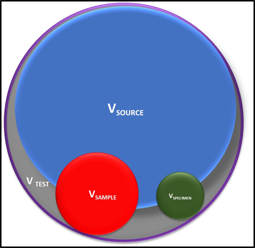
Sources of Variation. Homogeneity – the non-uniform distribution of microbes in the sample source (VSOURCE, where V = variability), the sample (VSAMPLE) and the specimen (VSPECIMEN) – contributes substantially to test result variability.
It’s Not the Method
A few years ago, a single set of fuel and fuel-associated water samples were used for two ASTM interlaboratory studies (ILS). You can read the details in the paper published in International Biodeterioration & Biodegradation. The ILS were performed based on the guidance provided by ASTM Practice D6300 for Determination of Precision and Bias Data for Use in Test Methods for Petroleum Products, Liquid Fuels, and Lubricants. As we discovered, D6300 is only applicable to properties that are both homogeneous and stable. Microbial contamination is neither. The two ILS were for ASTM Methods D7687 for Measurement of Cellular Adenosine Triphosphate in Fuel and Fuel-associated Water With Sample Concentration by Filtration and D8070 for Screening of Fuels and Fuel Associated Aqueous Specimens for Microbial Contamination by Lateral Flow Immunoassay. A few hours before the first ILS, specimens were prepared from samples known to have high, intermediate, and low bioburdens. Per D6300 a specimen was 200 mL fluid in a container, with three replicate containers for each combination of samples type (fuel grade or bottoms-water) and bioburden. Each container received a randomized code so that ILS participants would not know its contents. Preliminary ILS indicated that repeatability (single analyst) variability was < 5 % for each of the methods. Shockingly, the data from the D6300-based ILS indicated that both repeatability and reproducibility variability for each method were astronomical. I use the word shocking because both methods had long histories of yielding precise test results. The results suggested that the bioburdens in supposedly identical, replicate samples were actually substantially different. To test this theory, my collaborators and I compared the D7687 and D8070 results for each specimen. We found result agreement for 108 of 128 specimens (84 % agreement between methods). These findings inspired the development of ASTM Guide D7847 for Interlaboratory Studies for Microbiological Test Methods. The Guide enables ILS planners to reduce the variability of bioburdens in specimens so that test method rather than bioburden variability is tested.
In today’s What’s New article, I’ll explain some of the factors that contribute to test result variability. Remember that it is essential to understand test method variability before attempting to set data-based control limits.
Microbiological Test Result Variability – Are Microbes Present?
Are samples collected from locations most likely to have microbes?
In July 2021’s What’s New article, I wrote that the variability of microbiological test data is substantially greater than for other of tests used to analyze fuels, hydraulic fluids, lubricants, metalworking fluids (MWF), and other fluid samples. The non-uniform (heterogeneous) distribution of microbes in these fluids is often the primary factor contributing to test result variability.
The title Figure in today’s illustrates how non-uniform distribution of microbes within the system being sampled and the sample are typically the primary sources of variation. Typically, VSOURCE (where V = variability) increases as the ratio of oil (or fuel) to water increases.
The source is the system from which samples are collected. The most appropriate samples for microbiological testing are collected from places where microbes are most likely to accumulate in the system. I discussed this in some detail in the February 2020 What’s New article, and ASTM Practice D7464 provides detailed instructions for collecting samples intended for microbiology testing. The most accurate and precise microbiological test method will only detect microbes present in the test specimen – the volume or mass of material actually tested.
In most systems, bioburdens are most likely to be found on surfaces and at interfaces. It is important to understand that biofilms do not cover surfaces like coatings. Biofilms – either on system surfaces or at interfaces (i.e., the fuel-water interface) – are localized. Figure 1a shows biofilm accumulation in a fuel underground storage tank (UST). Biofilm of different thicknesses accumulate in bands along the UST’s length. Even though the nominal biofilm thickness within each band is rated by its average thickness (thick – ≥ 10 mm; moderate – ≥ 5 mm to < 10 mm; and minimal – < 5 mm), within the thick and moderate bands, biofilm thickness ranges from <0.1 mm to 10 mm. Consequently, the bioburden in replicates samples from adjacent 25 cm2 surfaces can vary by more than an order of magnitude. Similarly, Figure 1b shows the surface of a MWF sump. The heaviest biofilm accumulation is at the MWF-sump wall interface. However, as in the UST example, bioburden among replicate samples can vary by more than an order of magnitude. Figure 1c is a photo of two standpipe covers on the roof of a 5,000 m3 (30,000 bbl) diesel fuel above ground storage tank (AST). The distance between their respective centerlines is 16 cm. The AST bottom samples from the two standpipes (Figure 1d) are quite different in appearance and in their respective bioburdens.

Fig 1. Bioburden heterogeneity – a) UST bottom showing biofilm thickness zones; b) MWF sump wall showing biofilm thickness zones; c) 5,000 m3 diesel AST standpipe covers; d) bottom samples from the two standpipes shown in 1c.
Figure 2 illustrates bioburden heterogeneity in MWF (Figure 2a) and fuels (Figure 2b) respectively. The MWF is approximately 95 % water. Moreover, in an active MWF the fluid is recirculating at velocities sufficient to keep chips in suspension. Consequently, bioburden distribution in the MWF tends to be relatively homogeneous. Microbiology test results from replicate MWF samples typically vary by less than 20 %. In contrast, in fuel or oil samples that are nominally water-free, microbes tend to from discrete masses (flocs), making bioburden distribution in these fluids quite heterogeneous. The results from replicate samples can vary by more than an order of magnitude.
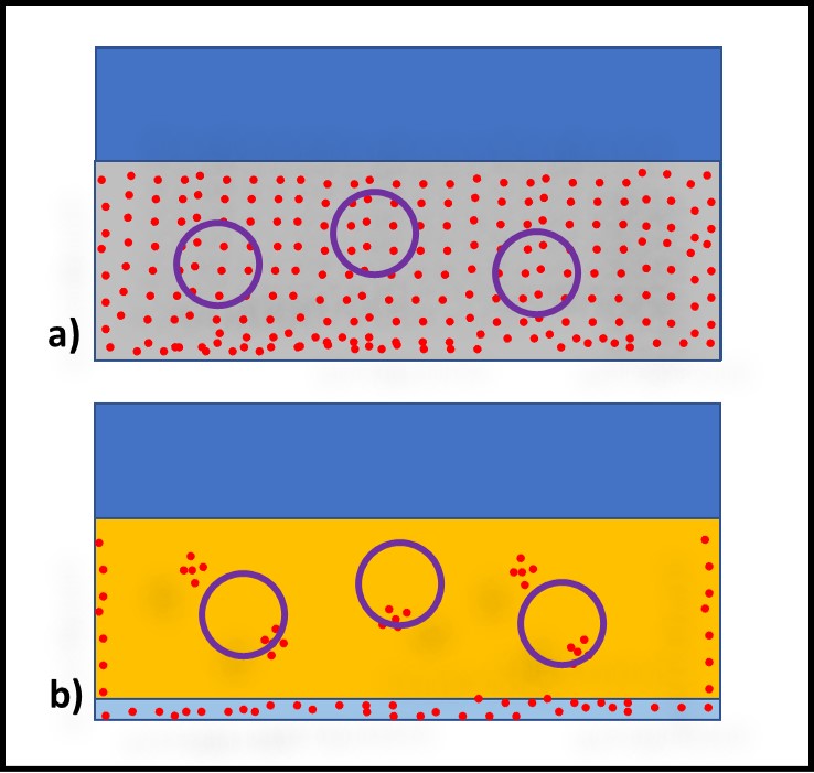
Fig 2. Source variability – a) MWF sump; replicate samples have similar bioburdens; b) oil sump (or fuel tank); replicate samples have different bioburdens. Red dots are microbes, purple circles are samples.
Are samples sufficiently large?
The VSAMPLE derives from VSYSTEM. As illustrated in Figures 1d and 2, bioburden heterogeneity in the system from which samples are collected contributes directly to bioburden differences among replicate samples. The purple circles in Figure 2 illustrate how the amount of bioburden captured in a sample bottle depends on bioburden homogeneity in the sampled fluid. Consequently, the results from triplicate samples of MWF are typically less variable than those from triplicate turbine oil samples.
One approach for reducing VSAMPLE is to increase the sample volume. Figure 3 illustrates how increasing the sample volume can decrease VSAMPLE. When bioburden distribution is uniform – as in recirculating MWF (Figure 3a) the bioburden per mL is unlikely to be affected substantially. However, when bioburden distribution is heterogeneous – as in oils and fuels (Figure 3b) – then increasing sample volume decreases the risk of failing to detect microbes present but heterogeneously distributed in the fluid.
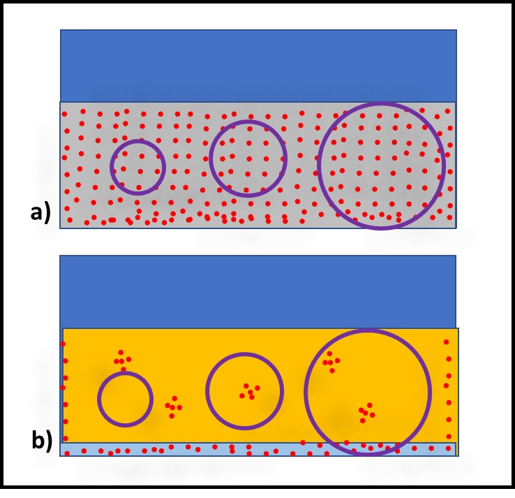
Fig 3. Sample size and microbe recovery – a) sample size does not affect bioburden capture in MWF; b) sample size substantially affects bioburden capture in fuels and oils.
Must the entire sample volume be tested?
The specimen is the portion of the sample that is tested. For example, for culture testing, the specimen size can range from <1 mL (ASTM Method D7978) to 500 mL (ASTM Practice D6974). The specimen size for adenosine triphosphate (ATP) testing by ASTM Method D7687 is either 20 mL of fuel or 5 mL of bottoms water, although, to increase test sensitivity, larger volumes are permitted. If 100 % of a sample is to be tested the specimen is equivalent to the sample and VSPECIMEN = VSAMPLE. Typically, however, the specimen volume is a small percentage of the sample volume. When this is the case, VSPECIMEN ≠ VSAMPLE. Figure 4 illustrates how VSPECIMEN is proportional to the bioburden’s heterogeneity in the sample.
For some fuel microbiological tests, the specimen is an extract from the sample. For example, ASTM Method D7463 uses 1 mL of a capture solution to extract polar molecules (e.g., whole cells, and polar organic – including ATP – and inorganic molecules) from the fuel phase. ASTM Method D8070 also includes an extraction step. For these methods, the efficiency with which the extractant transfers the analyte from the original sample contributes to VSPECIMEN.
As with the relationship between source and sample, the greater the sample’s water-content the more uniform the distribution of cells tends to be (Figure 4a). In nominally water-free fluids (Figure 4b) cell flocs tend to be distributed non-uniformly. Consequently, the bioburden in some samples is likely to differ from that in other samples. Vigorous shaking can reduce bioburden heterogeneity within a sample container. The amount of force used, and the duration of the shaking step will vary among sample types. Optimally, an adjustable, wrist-action shaker should be used (Figure 5). The wrist-action motion simulates hand shaking but eliminates the effects of fatigue – all samples are shaken with the same motion. The adjustment changes the amount of force imparted by each shake. Sample viscosity and the amount of flocing dictate the force needed to disperse microbes uniformly throughout the sample. If samples have multiple phases (e.g., fuel, invert emulsion, and free-water – Figure 6), the phases should be separated into different sample containers and then treated as separate samples for testing.
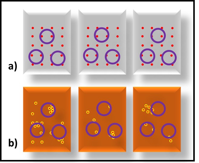
Fig 4. Specimen variability – a) MWF (aqueous fluid); b) turbine oil (viscous, non-aqueous fluid). The bioburdens in replicate specimens drawn from each of the MWF samples are less variable than those in replicate specimens from an oil or fuel sample. Red dots are microbes, purple circles are specimens.
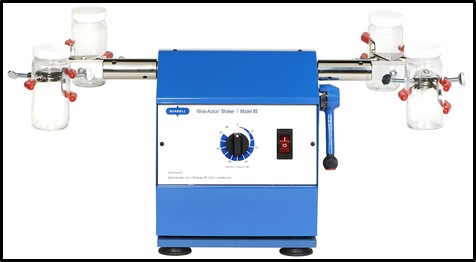
Fig 5. A four sample, adjustable force, wrist-action shaker. Both the range of arc and force applied for each cycle can be adjusted.
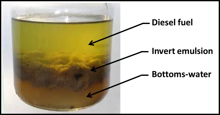
Fig 6. Three-phase sample from diesel UST. Before testing, phases should be separated, with each phase being transferred to a separate sample container.
A surface-active agent such as Cetyl Trimethyl Ammonium Bromide (CTAB) or Polyethylene glycol sorbitan monooleate (Tween® 80 – Tween is a registered trademark of Sigma-Aldrich), may added to samples to improve floc dispersion and bioburden heterogeneity in samples. The chemistry of the extraction reagents used for ASTM Methods D7463 and D8070 are proprietary. They are likely to contain one or more surfactants.
Last month I discussed quantitative recovery. In the article, I indicated that the essential element of quantitative recovery was consistency – regardless of whether the specimen preparation step recovered 5 % or 100 % of the analyte. In 2011, Defense Canada evaluated D7463’s extraction step. The data presented in Table 1 are taken from that study. For each sample, the ATP extraction step was repeated two to four times. The data were reported in relative light units per sample (RLU). The RLU in the second extracts ranged from 39 % to 137 % of the RLU in the first extract. Similarly, the RLU in the third extract ranged from ≤ 8 % (the test’s maximum RLU is 50,000) to 132 %. As I noted above, if the extraction step was quantitative, then RLU in subsequent extracts should have been a consistent fraction of the original. The fact that in some samples RLU in subsequent extracts were greater than in in the original and in other samples RLU decreased with each extraction demonstrated that the Method’s extraction step was not quantitative. The also means that VSPECIMEN was a major source of the method’s total variability.
Table 1. ASTM Method D7463 ATP extraction efficiency – middle distillate fuels.
| Sample | 1 | 2 | 3 | 4 | |||
| RLU | RLU | % | RLU | % | RLU | % | |
| 1 | 2,700 | 3,700 | 137 | 3,300 | 122 | N.D. | N.D. |
| 2 | 70 | 27 | 39 | N.D. | N.D. | N.D. | N.D. |
| 3 | >50,000 | 33,000 | ≤66 | 4,200 | ≤8 | 5,100 | ≤10 |
| 4 | 310 | 160 | 52 | 410 | 132 | 57 | 18 |
Microbiological Test Result Variability – Experimental Error
Experimental error includes the factors that contribute to protocol-related test result variability – VERROR.
Most commonly, VERROR reflects repeatability precision – the variability of replicate test results run on a single sample, by a single operator, using a single apparatus, over a short time period. The primary factors contributing to VERROR include:
- Effects of lot-to-lot reagent differences
- Testing conditions
- Operator’s skill
Effects of lot-to-lot reagent differences
All microbiological test methods use reagents. Stains are used for microscopic direct counts and flow cytometry. Nutrient media are used for culture testing. Extraction and bioluminescence reagents are used for ATP luminometry. Lot-to-lot variations in reagent composition can contribute to test result variability. Using ATP testing as an example, the RLU generated by a given concentration of ATP depends on the concentrations of Luciferase enzyme and Luciferin substrate in the luminescence reagent. Both components degrade over time. Consequently, the ratio of RLU to ATP concentration ([ATP]) decreases as reagent ages. Similarly, minor changes in growth medium nutrients and water concentration can affect the recovery of culturable microbes. Best practice is to routinely evaluate the impact of using different reagent lots, by running replicate tests using both the old and new lot reagents. This is a common practice in clinical labs but a rarity in industrial labs or among field operators performing condition monitoring tests.
Testing conditions
Enzymatic reaction rates vary with temperature. In 1889, his relationship was described mathematically by Svante Arrhenius. Figure 7 illustrates the logarithmic relationship between enzymatic reactions (including microbial growth rates) and temperature. Note that the y-axis scale is logarithmic. At temperatures greater than the one at which the reaction rate is maximal (Vmax) enzymes denature. Consequently, the reaction rate typically plummets as temperature continues to increase. The front end of the graph is important for microbiological testing. For example, the time needed for a bacterial colony to be visible will be longer at 20 °C than at 30 °C. If test kit instructions indicate that samples incubated at 30 °C should be observed at 48 h, but the actual incubation temperature is 20 °C, the results are likely to underestimate the actual CFU mL-1 (see What’s New, July 2017). Similarly, ATP test results are temperature dependent.
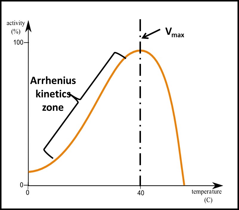
Fig 7. Enzymatic reaction rate – at temperatures less than the Vmax temperature, the reaction rate is described by the Arrhenius equation. At temperatures greater than the Vmax temperature, the reaction rate plummets as enzymes are destroyed and become inactive.
All testing should be performed at a standard temperature (for example 17 ± 2 °C – typical room temperature), or minimally at a given temperature. Using a reference standard reduces temperature’s impact on VERROR. In Figures 8 and 9, ATP was tested at 5 °C and 17 °C. The RLU at 5 °C were approximately 20 % of RLU at 17 °C (Figure 8). However, after raw RLU data were converted to [ATP] (pg mL-1) per ASTM D7687, the computed [ATP]s were statistically indistinguishable (Figure 9).
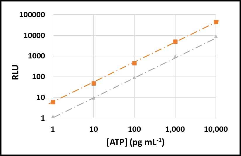
Fig 8. Temperature effect on ASTM D7687 results – orange squares: RLU at 17 °C; grey triangles: RLU at 5 °C.
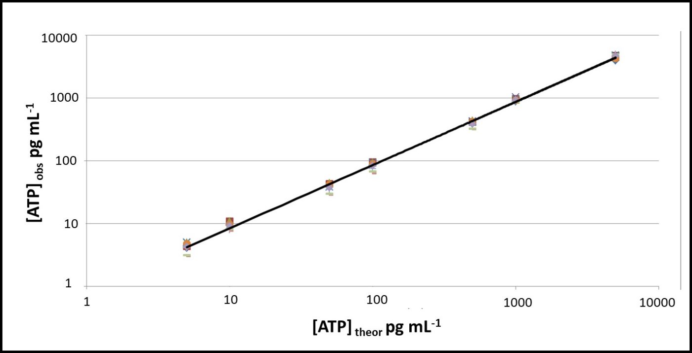
Fig 9. Temperature effect on ASTM D7687 results – orange squares: [ATP] at 17 °C; grey triangles: [ATP] at 5 °C.
Depending on the test method, other conditions such as gas composition (e.g., presence or absence of oxygen), relative humidity, and atmospheric pressure can affect results. However, these factors are rarely relevant for routine microbiological testing of industrial fluid samples.
Operator’s skill
Not long ago, an ILS (a different one form the one with which I opened today’s article) yielded surprisingly large reproducibility variation. Single-operator repeatability variation was negligible (< 5 %), but variability among labs was >2 orders of magnitude. The ILS coordinator performed a root cause analysis to help understand why the results varied so widely among participating labs. The investigation determined that none of the labs had actually followed the Test Method’s protocol steps. This experience highlighted the importance of operator training and quality assurance. Common operator factors that contribute to VERROR include:
- Sample handling
- Specimen collection and dispensing
- Reagent preparation
- Attention to protocol detail
Sample Handling – Operators must take precautions to avoid contaminating samples with microbes from their hands, the test facility environment, or devices used to handle samples. Earlier, I discussed the importance of agitating samples to homogenously disperse microbes. If the operator does not perform this step consistently (same amount of force for a standard time), the samples homogeneity will be affected. Homogeneity begins to degrade immediately sample agitation stops. The speed with which homogeneity degrades depends on the sample type. Best practice is to withdraw specimens within less than 1 min after agitating a specimen. If there will be more than a 1 min delay between specimens, the sample should be reagitated before the next specimen is drawn.
In multi-phase samples, bioburden tends to be much greater in the invert emulsion and aqueous phases. Failure to separate phases will cause higher bioburdens in those phases to bias (increase the apparent bioburden in) the fuel or oil phase test results.
Specimen collection and dispensing – the smaller the specimen volume the more critical it is to ensure that volumes are drawn and collected precisely. For example, for a 100 mL specimen, the impact of actually drawing 99 mL or 101 mL is 1 % to the total volume. In contrast, for a 10 mL sample the impact is 10 % and for a 1 mL sample it is 100 %. I have seen instances where a pipetting device was malfunctioning and an analyst – believing that they are transferring 1.0 mL of specimen – dispensed 0.0 mL. A high bioburden specimen was erroneously reported as having negligible bioburden. Pipetting devices vary on how they deliver fluid. Some are designed to deliver the designated volume although they retain some fluid. Others deliver the designated volume only when all fluid has been eliminated from the pipet. Operators must be sure that they are using pipets appropriately. They must also ensure that the entire specimen is delivered to the appropriate container. When specimens are being diluted, some methods prescribe that after dispensing the specimen into a solvent (or dilution blank) the pipet be rinses several times with the specimen-solvent mixture to maximized quantitative specimen transfer. Other methods do not prescribe this step. Operators must ensure that they perform this steps exactly as prescribed in each test method.
Reagent preparation – this step can be as simple as rehydrating freeze-dried reagents to following complex recipes. Any deviation from reagent preparation instructions can affect the test results substantially. During my undergraduate years, a visiting professor developed a nutrient medium with which he was able to cultivate a unique microbe that had never been recovered previously. After he published the research, others tried to reproduce his results. All were unsuccessful until the professor compared his lab notes with the published paper. The publisher had reversed the order in which they listed the growth medium’s ingredients. The switch made all the difference. Once other researchers started using the original recipe, they were able to reproduce the professor’s results. When preparing reagents, care must be taken to avoid infecting them with microbial contaminants. Operators must also be careful to follow reagent storage requirements (e.g., store in the dark, within a specified temperature range, for no longer than the specified period).
Attention to protocol detail – as I mentioned regarding the ILS with the excellent repeatability variation but horrible reproducibility variation, it is imperative that operators follow the protocol precisely as prescribed. Field tests are typically more forgiving than laboratory tests in this regard. Test kit manufacturers invariably invest substantial time and effort to understand the factors that affect their kit’s precision and accuracy. Similarly, researchers who publish peer-reviewed methodology papers understand the non-analyte factors that can affect test results. New operators often need training on how to perform manual tasks such as sample shaking, pipetting, calibrating instruments, etc. Performing protocol steps improperly can contribute to imprecision, in accuracy or both.
Summary
Microbial contamination in industrial systems can be localized. One consequence of this localization is that samples collected from heavily contaminated systems can be microbe-free. By extension, microbiological test methods will not detect microbes that are not captured in a sample. The heterogeneous distribution of microbes also means that VSYSTEM and VSAMPLE can be much greater than any test method’s VERROR. Notwithstanding the heterogeneity issue, improper sample handling contributes to VSPECIMEN and sloppy performance of microbiological tests contributes to VERROR. Following best practices for identifying appropriate diagnostic sample collection points and sampling protocols decreases the risk of failing to detect microbial contamination in infected systems. Proper sample handling and test method performance improve test result accuracy and precision.
As always, I look forward to receiving your questions and comments at fredp@biodeterioration-control.com.
