MICROBIOLOGY FOR THE UNITINTIATED – PART 6: BACTERIA

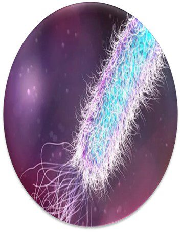
A rod-shaped, polarly flagellated bacterium.
Source: https://factrepublic.com/facts/33765/

Introduction

Now that I’ve provided an overview of the characteristics of all life, I’ll describe the most common types of organisms that contaminate industrial process fluid systems – i.e., oilfield injected and produced waters, fuel-associated waters, heat exchange systems, and countless other systems in which fluids are contained of through which they flow. Historically, the two primary types of microbes recovered from systems not exposed to light are bacteria and fungi. More recently a third group – archaea – have been detected too. When light is present, algae are common contaminants. In this article I’ll discuss bacteria. In future articles I’ll focus on each of the other types of microbes.

The Tree of Life

Taxonomy is the science of classifying living things. In 1735, Carl Linnaeus published Systema Naturae in which he described a binomial system for identifying plants (i.e., originally plant and subsequently all organism based on whether they shared or didn’t share a characteristic). Under Linnaean taxonomy, there are eight categorical levels (Figure 1). The highest – most inclusive – level is domain. As illustrated in Figure 3a, there are three domains – Bacteria, Archaea, and Eucarya. Each domain is divided into Phyla. Thus far, the domain Bacteria has approximately 1,300 phyla – with the number still increasing. Phyla are further divided among classes. Again, using Bacteria as our example, the phylum Proteobacteria is comprised of five Classes – Alphaproteobacteria (α-proteobacteria), Betaproteobacteria (β-proteobacteria), Gammaproteobacteria (γ-proteobacteria), Deltaproteobacteria (δ-proteobacteria) and Epsilonproteobacteria ( ε-proteobacteria). The γ-proteobacteria includes 14 Orders which are further divided into 404 Families. For example, the Order Pseudomonadales includes two Families – Moraxellaceae and Pseudomonadaceae – both of which include bacteria commonly recovered from industrial process water systems. Families are comprised of genera (singular – genus). Thus, the genus Pseudomonas is a member of the family Pseudomonadaceae. Traditionally, species was the smallest taxonomic unit (for example Pseudomonas aeruginosa). However, current taxonomic schemes typically include two additional levels – strains and biovariants (abbreviated as biovar.).

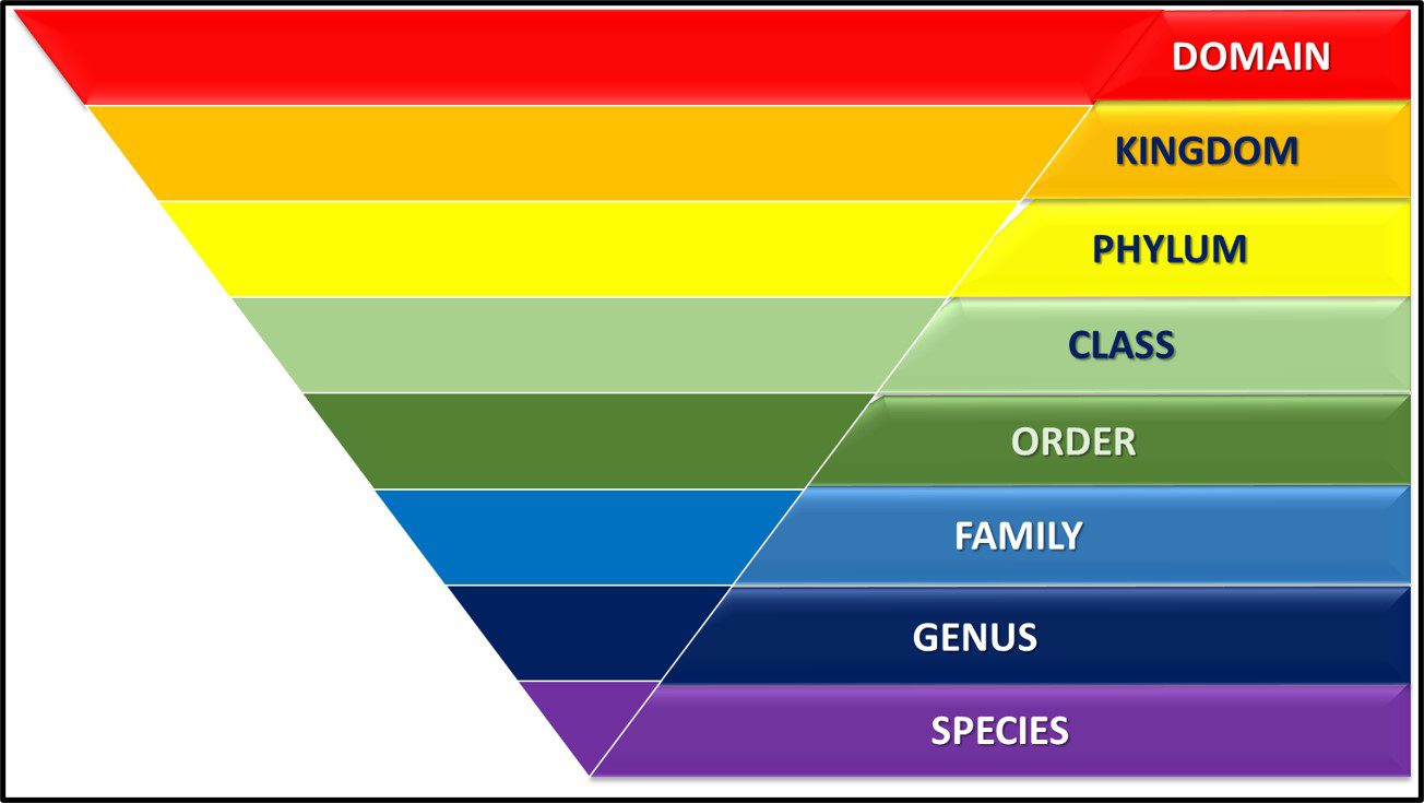
Fig 1. Linnaean taxonomy’s eight taxonomic levels.

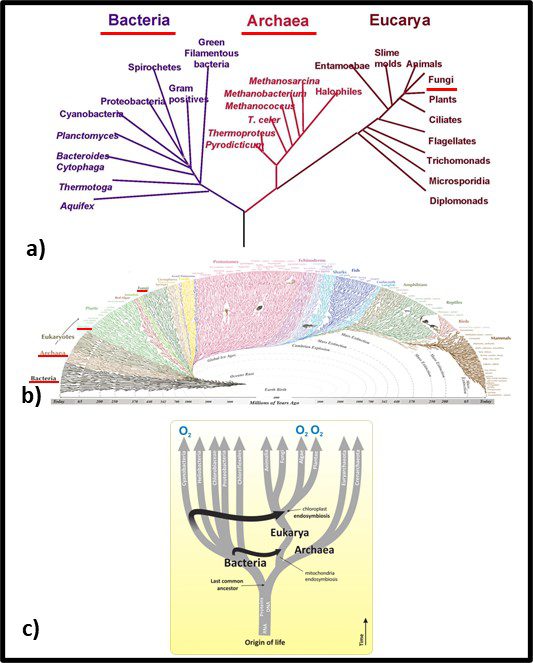
Fig 2. Phylogenic trees – a) simplified tree showing genetic distances between Bacteria, Archaea, and Fungi; b) more complex genomic map illustrating Bacteria’s emergence approximately 3.2 billion years ago, Archaea’s emergence approximately 1.5 billion years ago, and fungi arriving at approximately the same time as vascular plants – approximately 1 billion years ago. Sources: a) Carreón, Gustavo & Hernández-Zavaleta, Jesús Enrique & Miramontes, Pedro. (2005). DNA Circular Game of Chaos. 757. 10.1063/1.1900503, b) https://i.pinimg.com/originals/46/28/92/46289232f53138d4134ea0e829589d09.gif, c) https://organismalbio.biosci.gatech.edu/biodiversity/eukaryotes-and-their-origins/.

In traditional taxonomy – including microbial taxonomy – organisms were clustered based on their observable similarities. Thus, members of a genus share more characteristics than members of a family. Diversity increases with the classification level. Currently, microbial taxonomists estimate there are at least a billion bacterial species, of which fewer than 10,000 have been characterized (that’s <0.001 % in case you are wondering). Figure 1b offers a visual perspective on the diversity of bacterial life. The black, web-like region on the bottom left reflects the genetic branching since bacteria first existed – an estimated 3.2 billion years ago (the Earth’s estimated age is 4 billion years). I don’t expect readers to use Figure 2b as anything more than an illustration of just how divers the kingdom Bacteria is. Figure 1c provides a simplified tree showing first the evolution of eukaryotes as hosts for bacteria and second the similar age of the Archaea and Eukaryote domains. Figure 3c also illustrates how genetic material (ribonucleic acid – RNA, deoxyribonucleic acid – RNA, and proteins were probably components of self-replicating proto-microbes before the last universal common ancestor (LUCA). Based on genomic analyses, the LUCA is estimated to have existed between 3.48 and 4.1 billion years ago – soon after Earth formed. Although the term LUCA suggests that there was a single genetic entity from which all subsequent life evolved, it is more likely that numerous types of protomicrobes developed and the most successful continued to evolve.

What are Bacteria?

ASTM provides a good working definition. A bacterium is any member “of a class of microscopic single-celled organisms reproducing by fission or by spores. Characterized by round, rod-like, spiral, or filamentous bodies, often aggregated into colonies or mobile by means of flagella. Widely dispersed in soil, water, organic matter, and the bodies of plants and animals. Either autotrophic (self-sustaining, self-generative), saprophytic (derives nutrition from nonliving organic material already present in the environment), or parasitic (deriving nutrition from another living organism).” I discussed bacterial reproduction in July 2023.

By current estimates, Bacteria are the most diverse organisms. To paraphrase Donald Rumsfeld’s “Known knowns” comment, bacterial diversity and total biomass estimates fall into the category of known unknowns. Figure 3 illustrates a typical dendogram created from DNA data from a soil sample. The dendrogram’s branches represent genetic similarities, with similarities between two DNA molecules increasing as the dendogram branches from left to right. Most commonly, the individual organism type – operational taxonomic units (OTU) are identified only by alphanumeric codes. This is because only a small percentage of bacterial OTU that have been detected by genomic profiling have been identified at the Family, Genus, or Species levels. During the past decade, some researchers have suggested that apparent similarities among DNA molecules based on their migration through an electric field gel (denaturing gradient gel electrophoresis – DGGE – see the black bands in the center of Figure 3) is misleading. DNA molecules with different genes can appear to be common OTUs. Some have argued the amplicon sequence variant (ASV) is more precise. Repeating my mantra, I make this point only to illustrate my point about bacterial diversity. As I explained in my July 1018 What’s New article, unlike antibiotics which are designed to kill specific microbes without damaging surrounding human cells (or microbes that are essential for good health), industrial microbicides typically target a broad spectrum of microbes. My favorite analogy is Bambi v. Godzilla (Figure 4). Full taxonomic profiles can be useful to understand the microbial ecology of the system under investigation, but is unlikely to inform contamination control decisions.

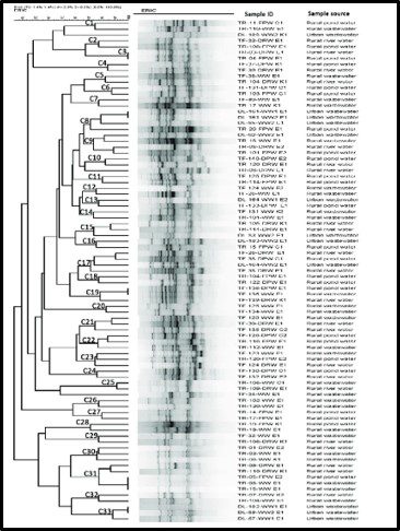
Fig 3. Dendogram of genomic profile of bacteria recovered form water samples. Source: https://journals.plos.org/plosone/article?id=10.1371/journal.pone.0261970

Fig 4. Bambi versus Godzilla (Source: 1969 animated feature – https://www.indiewire.com/2015/01/a-bambi-meets-godzilla-live-action-remake-123687/#!)

Classifying Bacteria

Shape

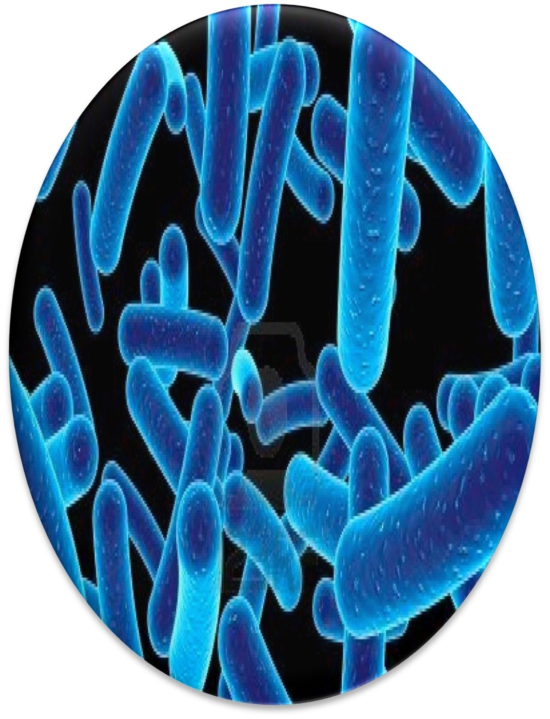
Recognizing that the microscope was the first tool use to detect and identify bacteria, the earliest taxonomic schemes were based on their appearance (morphology). With variations within each group, the primary forms are rod, spheres, commas, and spirals (Figure 5). Once the Gram stain – developed by Hans Christian Gram – was able to differentiate between bacteria with cell walls thet retained an iodine-based stain and those that didn’t – bacteria in each of the morphological groups were classified as being either Gram positive (Figure 6a) or Gram negative (Figure 6b).

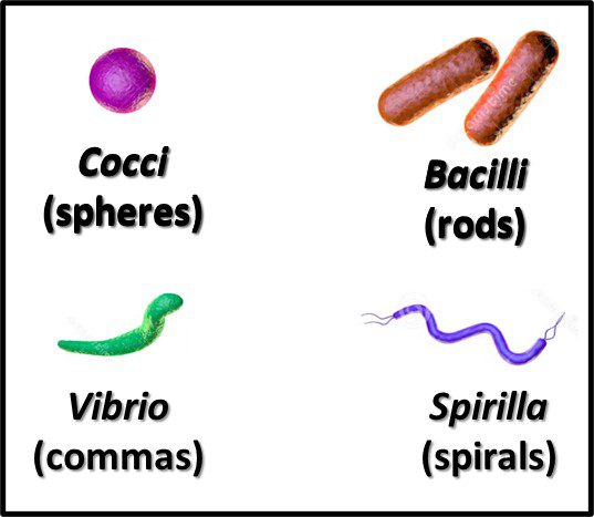
Fig 5. Primary bacterial morphologies.

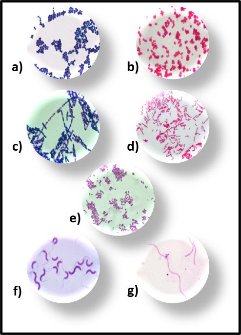
Fig 6. Primary bacterial morphologies after Gram staining – a) Gram positive rods; b) Gram negative rods; c) Gram positive spheres; d) gram negative spheres; e) Gram negative commas; f) Gram positive spirals; and g) Gram negative spirals.

It would be decades before the biochemical basis for Gram positive and Gram negative reactions were understood. As illustrated in Figure 7, the Gram positive cell walls are structurally less complex from those of Gram negative bacteria. The largely carbohydrate Gram positive cell wall retains the iodine stain. The peptidoglycan structure of Gram negative cells do not. Other groups of microbes have subsequently been classified based on their reactions to specific stains (acid fast stain, spore stain, etc.).

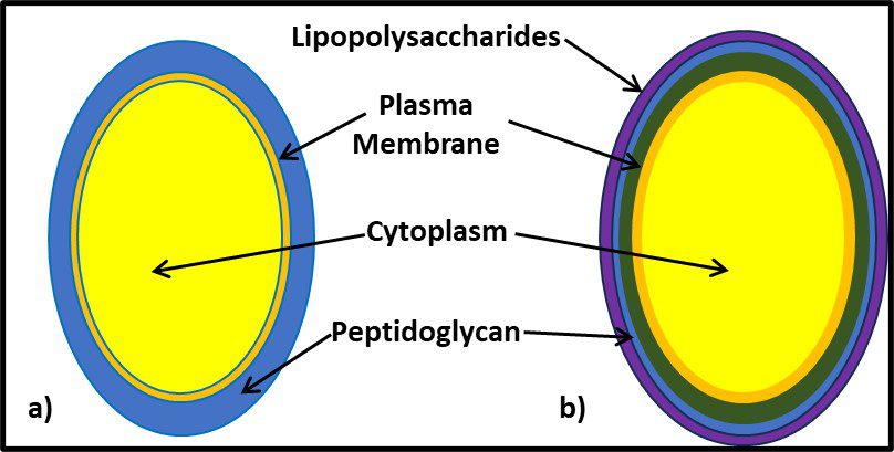
Fig 7. Cell wall structure – a) Gram positive cell (mostly peptidoglycan); b) Gram negative cell (the cell wall is substantially more complex; the peptidoglycan layer is covered by a lipopolysaccharide layer).

Although morphology can be a useful tool, it is limited due to bacterial pleomorphism – the ability of a specific microbe’s shape to change in response to its environment. More that 20 years ago, researchers at University of Montana’s Center for Biofilm Engineering demonstrated that during biofilm development both the morphology and physiology of genetically identical cells varied, depending on where cells were located within the biofilm matrix. I’m not sure why this was such a startling discovery. Just consider the morphological and physiological diversity of human cells, depending on where they are in (or on our bodies – Figure 8).

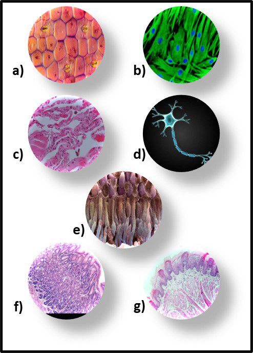
Fig 8. Human tissue cells – a) epidermis (skin); b) hair follicle cells; c) lung cells; d) nerve cell; e) retinal cells; f) stomach cells; g) tongue cells.

Physiology

Before genetic testing became affordable and readily accessible, physiological tests were the primary tool – after morphology – to identify microbes. Physiological testing profiles a microbe’s ability to utilize specific nutrients (e.g., glucose or other sugars, various amino acids, hydrocarbons, etc.), produce characteristic metabolites (e.g., ethanol, acetic acid, various gases, etc.), or grow under particular conditions (e.g., oxic or anoxic; acidic, neutral, or alkaline; cold, temperate or hot; etc.). A full battery of physiological tests can include more than 400 different conditions. Traditional microbiological taxonomy standards (for example, Bergey’s Manual of Determinative Bacteriology – nine editions published between 1923 and 1994 – was long considered to be the bible for bacterial identification).

One underappreciated limitation of physiological testing is that these tests could only be run on microbes that could be cultivated in the first place. Moreover, the physiological capabilities of a pure culture can vary with the culture’s age. Consequently, cultures are subject to misidentification due to the variations in their physiological properties as a function of age. I one project, I sent specimens from a single colony to several different labs. Although all the labs used the same automated physiological testing equipment, each lab reported different identities for the culture. When specimens of the same culture were sent to several labs for genetic testing, all identified the microbe correctly.

That said, grouping microbes into physiological classes to assess biodeterioration risk can be useful. I routinely run BART™ (BART – Biological Activity Reaction Test – is a trademark of Droycon Bioconcepts, Inc., Regina, Canada) tests on fuel or fuel-associated water samples that have high ATP-bioburdens. BART vials each contain one of nine different dried media. I typically test for acid producing bacteria (APB), iron related bacteria (IRB), denitrifying bacteria (DN), nitrifying bacteria (NB), slime-forming bacteria (SLYM), and sulfate reducing bacteria (SRB) – microbes commonly associated with microbiologically influenced corrosion. Figure 9 illustrates the reactions in APB, IRB, SLYM, and SRB BART vials inoculated from fuel-associated water.

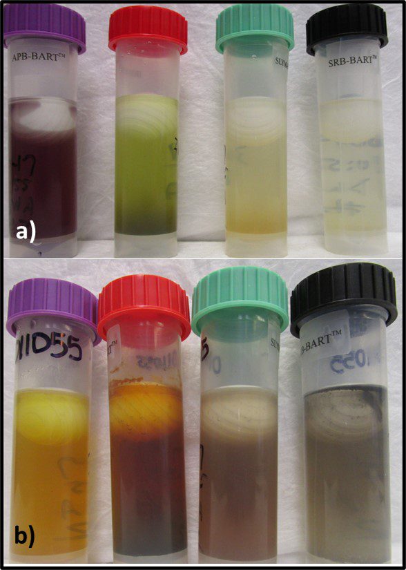
Fig 9. BART (left to right) APB, IRB, SLYM, and SRB vials inoculated with fuel-associated water – a) Immediately after inoculation; b) after 4-days incubation. The sample was positive for all four metabolic groups.

Figure 9a shows the vials’ appearances immediately after inoculation. Figure 9b shows how each vial changed color and became turbid after four-days’ incubation. The microbes growing in each vial represented diverse types of individual taxa that shared a physiological property – i.e., acid production, etc.

Similarly, representatives from diverse taxa are included in each respiration and fermentation category (see August 2023). Classifying microbes based on their ecologically important physiological properties is like classifying trades people based on their skills – carpenters, electricians, plumbers, welders, etc. It provides no indication of their family lineages.

Optimal and Tolerated Growth Conditions

Just as genetically diverse microbes fall into different physiological categories, they also fall into different growth condition categories. Here, I’m using growth condition to include environmental factors such as temperature, pH, and salinity.

Temperature

Psychrophilic bacteria grow optimally at temperatures between 10 °C and 15 °C. Most will not grow at temperatures >20 °C. Mesophiles – the microbes most commonly associated with disease – require moderate temperatures in the 20 °C to 40 °C range. Most bacteria isolated from fuel and industrial process fluid systems where temperatures are typically <45 °C are mesophilic. Thermophiles require hotter temperatures (≥45 °C). Thermophiles have been recovered from environments where the temperature is >100 °C. Figure 10 illustrates how microbes are classified based on the temperature range in which they will grow.

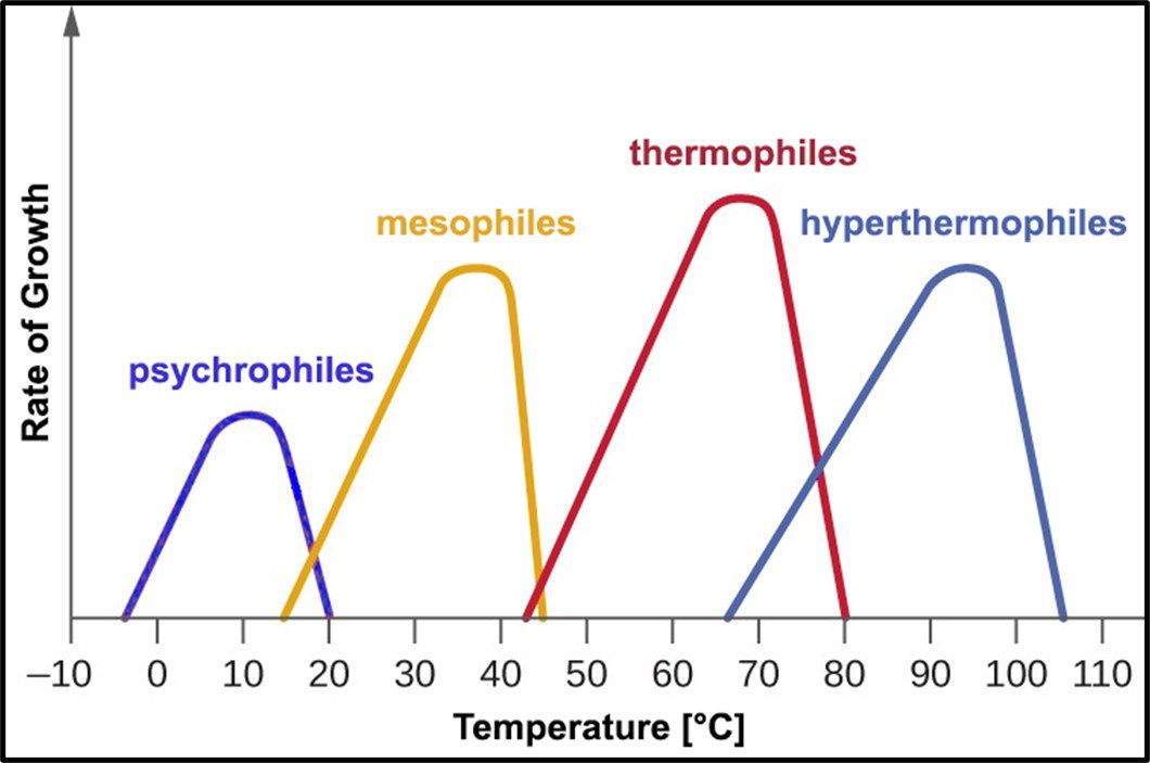
Fig 10. Microbe classification by optimal and tolerated temperatures.

pH

The Mirriam-Webster online dictionary defines pH as “a measure of acidity and alkalinity of a solution that is a number on a scale on which a value of 7 represents neutrality and lower numbers indicate increasing acidity and higher numbers increasing alkalinity and on which each unit of change represents a tenfold change in acidity or alkalinity and that is the negative logarithm of the effective hydrogen-ion concentration or hydrogen-ion activity in gram equivalents per liter of the solution.” Mathematically,

Where “p” is a term with an interesting history (which I won’t share here). In water, the fractional sum of hydrogen (H⁺) and hydroxide (OH^–) ions is always 1. As shown in Figure 11, pH decreases as Log₁₀ [H⁺] increases. At neutral pH, Log₁₀ [H⁺] = Log₁₀ [OH^–]. Neutrophiles only grow when the in the pH range 7 ± 1.5. Acidophiles thrive at lower pHs. Some (extreme acidophiles) grow in water with pH = 1. Conversely, alkalinophiles require pH ≥ 9 (Figure 12).

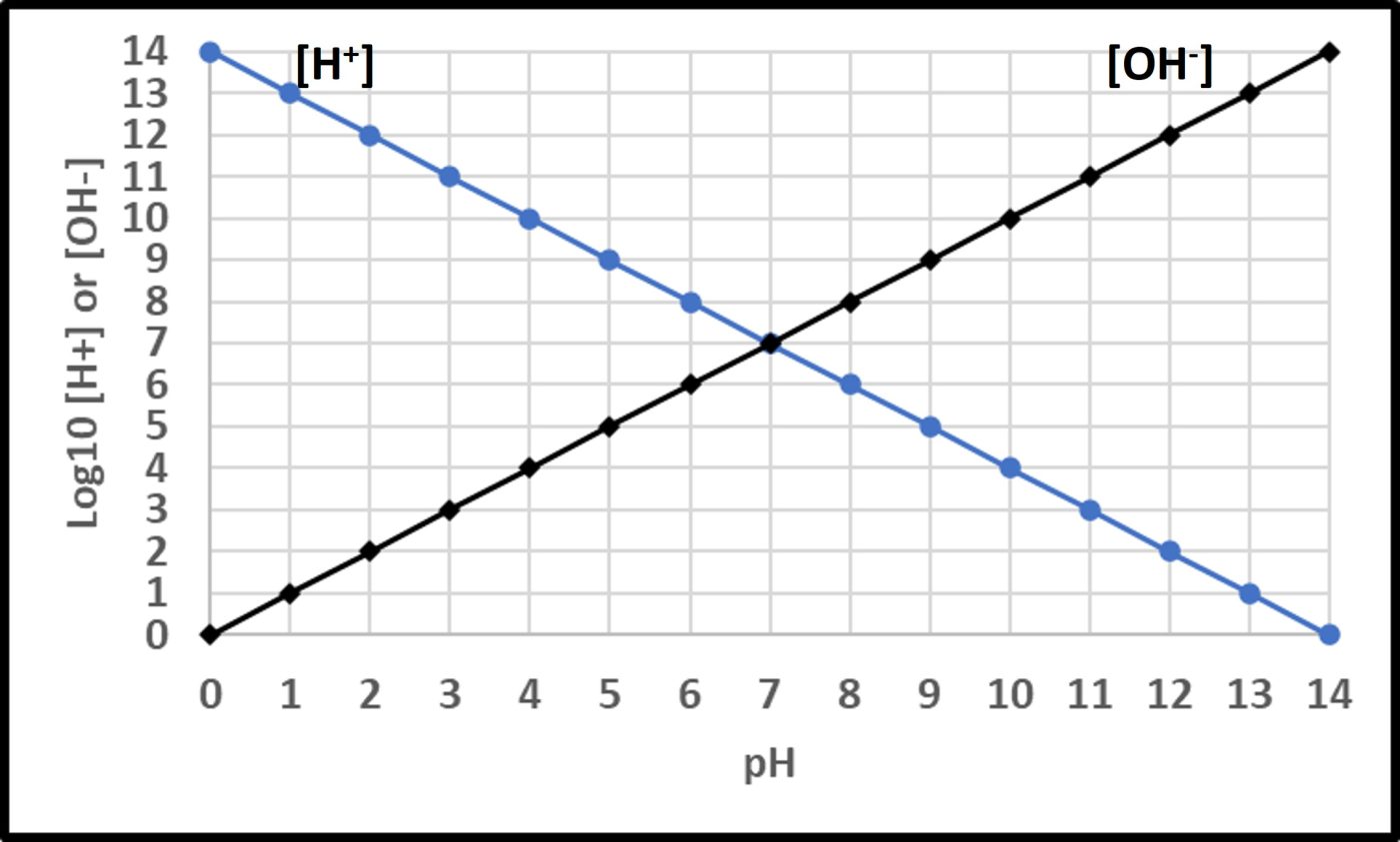
Fig 11. Relationships between hydrogen ([H⁺] and hydroxyl ([OH^–]) ions and pH.

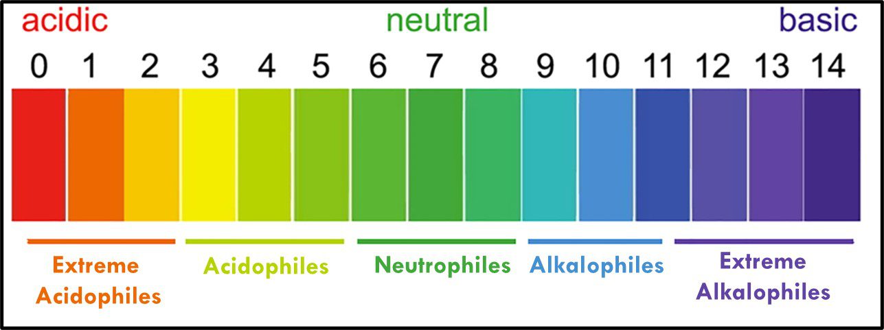
Fig 12. Microbe classification by optimal and tolerated pH ranges.

Other environmental conditions

Microbes can also be classified based on their preference (i.e., condition for optimal or maximal growth) for atmospheric pressure (barophiles only grow in environments with pressures ≥ 10,000 kPa (100x atmospheric pressure, and vacuumphiles grow in environments with pressures in the 5 kPa to 15 kPa range – 0.05x to 0.14x atmospheric pressure), osmotic pressure, salinity, radiation, or other factors that span ranges that select for different microbes at different requins of the parameter’s range. Organisms that prefer life at the high or low ends of each factor are called extremophiles. Some types of microbes enjoy environments that are extreme by more than one criterion. For example, microbes thriving around deep-sea ocean vents are thermophilic barophiles. They require both high temperatures and pressures.

Most higher life forms can tolerate only a narrow (in Goldilocks terms – just right) range of each of these factors. Bacteria and archaea are unique in the range of environmental conditions they enjoy as kingdoms. However, individual taxa are limited in the range of environments in which they can thrive. Still each time a group of scientists report they have discovered an environment on Earth that is completely devoid of life, they are proven wrong. The development of genetic testing has made it possible to detect bacteria and archaea (more on archaea in my next article) that had previously been undetectable. Regarding the ability of one or more life forms to exist in Earth’s most hostile environments, Carl Sagan’s adage – “The absence of evidence is not evidence of absence” – has been proven true. Of course, Professor Sagan was referring to life beyond earth. We will have to wait and see on that front.

Summary

The domain Bacteria is genetically the most ancient and diverse of the three domains into which all life on earth is divided. To date, microbiologists estimate that we have detected <0.001 % of the different types of bacteria thought to exist in nature. Although the tools used to traditionally identify bacteria are still of some value, genomic test methods have changed the game. Microbes that once seemed to be closely related, based on their appearance and nutritional characteristics (physiology) have been shown to be genetically distant. Conversely, other microbes, once thought to be dissimilar are now known to be close genetic relatives. Because of their ecological and physiological diversity, bacteria play major roles in biotransformation processes (I’ll write about nutrient cycles in future What’s New articles). When biotransformation causes damage, we call it biodeterioration. When it is used to produce useful products, we call it biotechnology, and when it facilitates remediation, we call it bioremediation. We need to remember that microbes live their lives unaware of the labels we humans apply to their activities.

In this article I have barely scratched bacteriology’s surface. Quite often clients ask me to provide them with a list of microbes present in a contaminated system. I invariably ask what they will do with that information. In my opinion, the art and science of microbial contamination control depends on understanding what the population is doing rather than identifying taxonomic names. What do you think? As always, please share your comments and questions with me at fredp@biodeterioration-control.com.

STLE’S TRIBOLOGY & LUBRICATION TECHNOLOGY JUNE 2023 ISSUE SOUNDING BOARD

Bacteria
Source: BACTERIA – Bing images

June TLT Sounding Board Question 1: “Do you think that biolubricants are more sensitive to microbiological attacks?”

In Talmudic style, my response to that question is another question: is biolubricant susceptibility to microbial attack – i.e., biodeterioration – a matter of conjecture?! Most of the respondents apparently thought so. However, one responded: “Depends on the composition and overall resistance to microbial attack. I would imagine testing on microbial resistance would be part of the testing for new products.” This individual chose not to take the bait. They recognized that “sensitivity to microbial attack” depended on the finished stock’s chemistry rather than its source.

Having it both ways?

As ASTM D8324 Standard Guide for Selection of Environmentally Acceptable Lubricants for the U.S. Environmental Protection Agency (EPA) Vessel General Permit points out, the concept of an environmentally acceptable lubricant (EAL) aligns with Humpty Dumpty’s comment: “When I use a word,’ Humpty Dumpty said in rather a scornful tone, ‘it means just what I choose it to mean — neither more nor less.’” Figure 1’s exchange between Humpty Dumpty and Alice is relevant for several reasons.

1. There are numerous EAL labels and the criteria for each label is unique. Germany’s Blue Angel, EU’s Ecolabel US EPA’s EAL, respective criteria are similar but different criteria. Thus, the concept of what defines an environmentally friendly lubricant is a matter of debate.

2. Alice’s response is a question all too commonly asked by marketers. One common trope among companies selling water-miscible metalworking fluids (MWF) is the claim that their product is “biocide-free” when it most likely contains an unregistered component that’s more toxic than most registered biocides (see What’s New, February 2022).

Fig 1. Humpty Dumpty’s perspective on definitions.

3. Humpty Dumpty’s retort is again relevant to the extent that folks can use meaningless generalizations to support any point of view. The fact is that biolubricant biodegradability can and has been tested.

Lubricant marketers want to be able to claim that their products are environmentally acceptable, but are considerably less enthusiastic about also claiming that readily biodegradable products are – well – also readily susceptible to biodeterioration.

Biodegradability testing

All of the environmental label issuers require biodegradability testing. Typically testing is performed in accordance with Organisation for Economic Co-operation and Development (OECD) Test 301 OECD Guideline for Testing of Chemicals – Ready Biodegradability. OECD 301 has a number of variants – 301A through 301F. As illustrated in Figure 2, the first step is to determine a product’s partition coefficient (OECD 117). If the product’s n-octanol/water partition coefficient – P_OW (P_OW = ; Log P_OW = K_OW) – is in the ≤3 K_OW ≤ 7 range, then the substance is potentially bioaccumulative. Bioaccumulative substances are those that can be captured irreversibly in the tissues of various organisms. When K_OW is in the 3 to 7 range, the next step is to test for biodegradability. Lubricants are biodegradable if > 95 % (^w/_w) of the formulation is biodegradable (>70 % of each molecular species is mineralized within 28 days). If >5 % of the formulation is not biodegradable, the product is then tested in accordance with OECD 305 Bioaccumulation in Fish. The key points here are:

1. Biobased feed stocks and lubricants can readily be tested for their partition coefficient, and

2. If K_OW is in the 3 to 7 range, the lubricant’s water accommodated fraction can be further tested for biodegradability.

There is no need to speculate about biobased lubricant biodegradability (i.e., susceptibility to microbiological attack). The OECD test methods are standardized, making it possible to compare how readily any finished lubricant or lubricant stock might be.

Fig 2. A very simplified flow chart for assessing lubricant or lubricant base stock biodegradability and bioaccumulative properties.

Keep in mind that if there is no water present, then neither lubricants nor base stocks – regardless of their chemistry – will be susceptible to microbiological attack. Similarly, if none of the lubricant or base stock partitions into the aqueous phase when water is present, it is not going to be susceptible to microbiological attack.

Here’s the having it both ways conundrum: by definition, the more biodegradable a substance by OECD 301, the more susceptible it is to microbiological attack. Ecological good news is necessarily operational bad news unless you keep water out of the lubricating system!

Are all biobased stocks equal?

Fatty acid methyl ester (FAME) is used to blend biodiesel fuels. Consequently, FAME biodegradation susceptibility has been studied quite extensively. It is not unreasonable to use FAME biodegradation knowledge as a starting point to speculate about biolubricant basestock resistance to microbial attack.

Generally speaking, biodegradability inversely related to oxidative stability. The primary factors affecting both oxidative stability and bioresistance are carbon chain length and saturation. FAMEs with shorter chain length (i.e., <C ₁₅) tend to be more biologically and oxidatively stable than those with chain lengths > C₁₅. Also, saturated molecules (i.e., those with no carbon-carbon double bonds – C=C) are more stable than mono- or polyunsaturated carbon chains (Figure 3). Note, for example that coconut FAME (C₁₂-C₁₄; >85 % saturated) is quite stable. It is even used as a topical antimicrobial agent. Conversely soy and canola FAME (are composed of primarily C₁₆-C₁₈ and C₂₄-C₂₆ mono- and polyunsaturated acids – soy is ~14 % saturated and ~canola is 5 % saturated). Both are readily biodegradable.

Fig 3. Relative biodegradability of selected biobased oils and fatty acid methyl esters.

Summary

Biobased lubricants and lubricant stock susceptibility to biodegradation should not be assessed by polling. As my friend and STLE Metalworking Fluid Education Committee colleague John Burke frequently observes, “without data, you are just another person with an opinion.” Everybody has an opinion, but objective data are relatively easy to develop. The question should have been the basis of a research effort rather than an opinion poll.

What do you think? As always, please share your comments and questions with me at fredp@biodeterioration-control.com.