MICROBIOLOGY FOR THE UNITINTIATED – PART 9: ARCHAEA
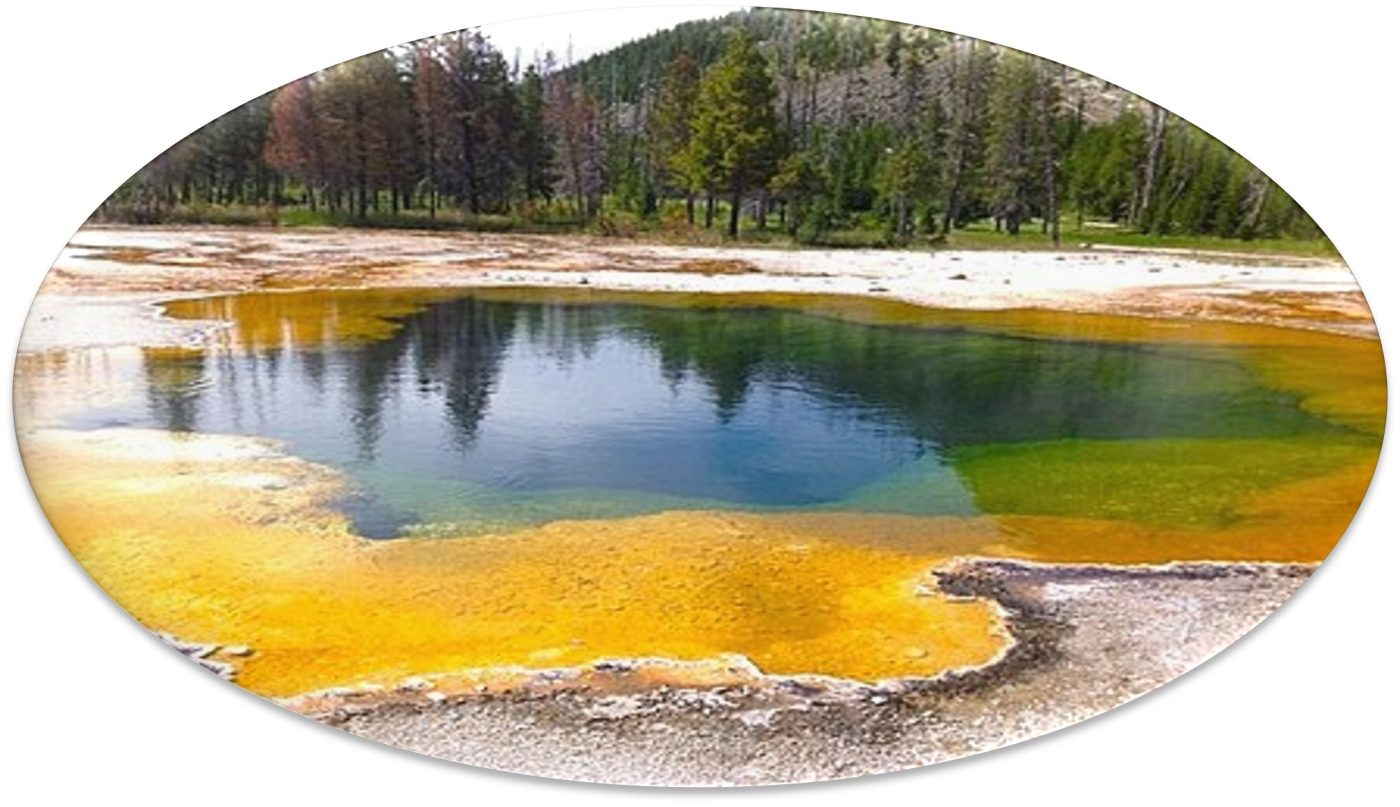
Mats of Archaea on surface of Morning Glory hot spring, Yellowstone Park, WY. Source: 440px-Morning-Glory_Hotspring.jpg (440×328)
Introduction
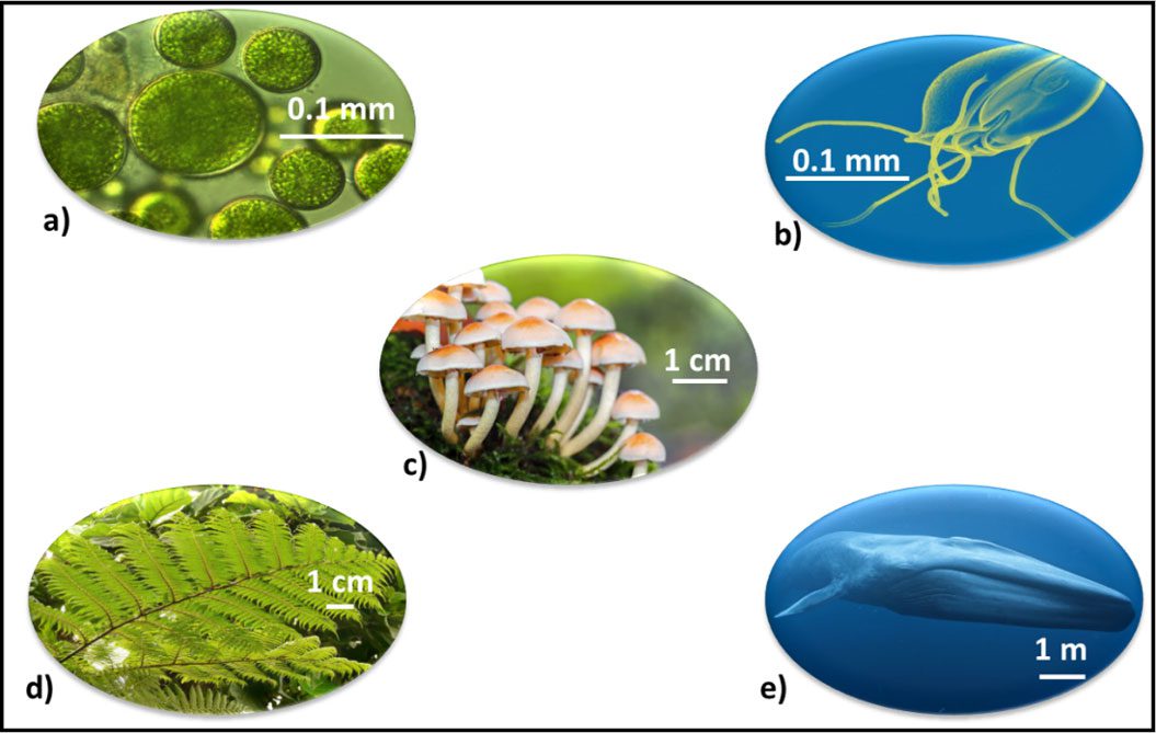
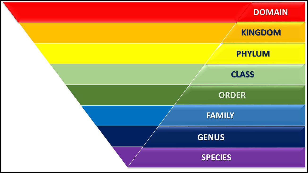
From the 1860s through the 1970s, the tree of life was grouped into three domains – Plantae, Protista, and Animalia1 (Figure 1).
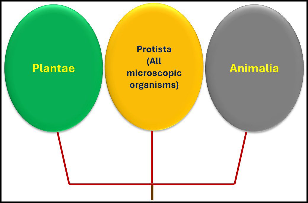
Fig 1. Simplified phylogenic tree based on Haeckel, 1866.
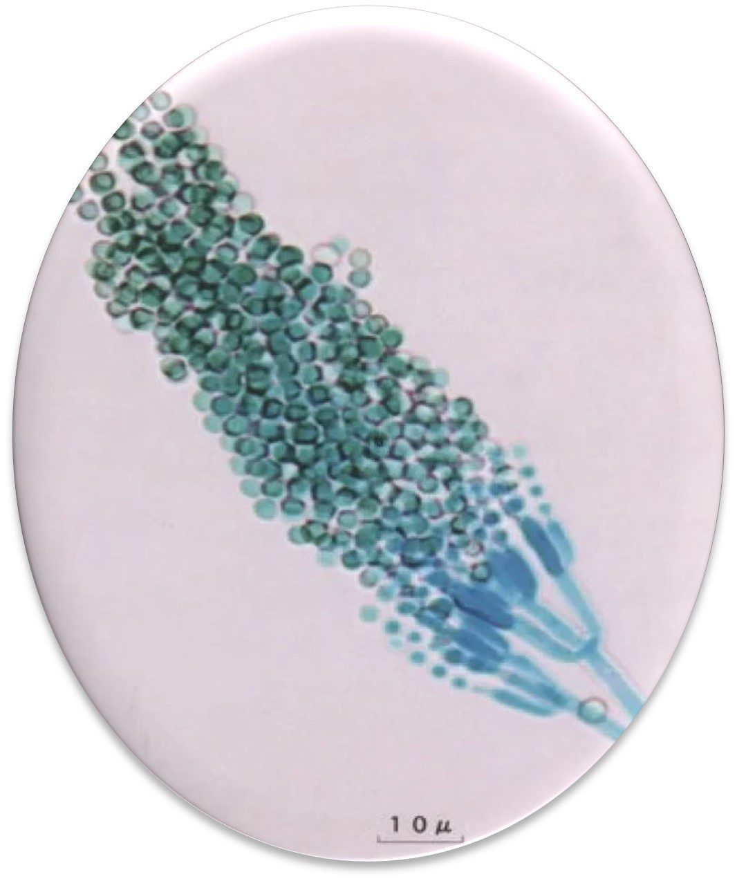
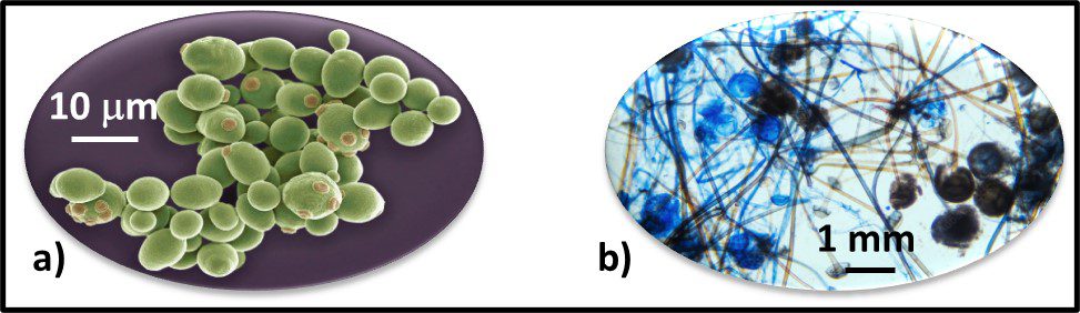
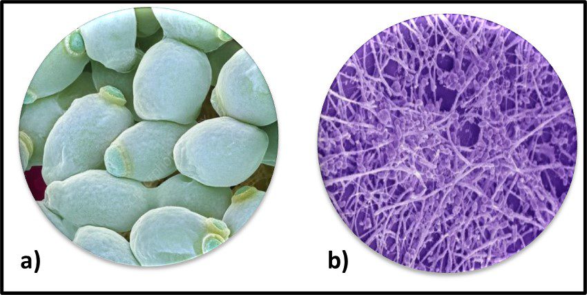
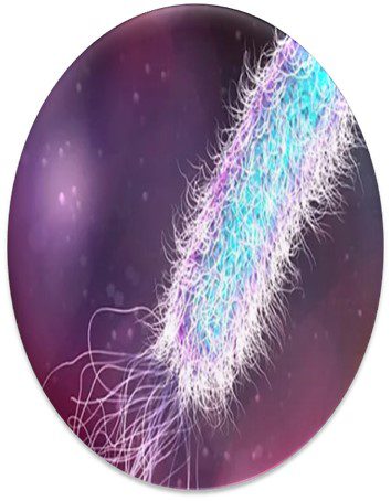
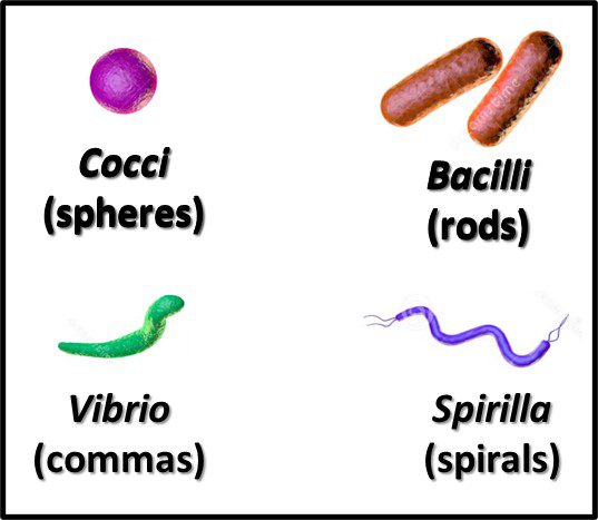
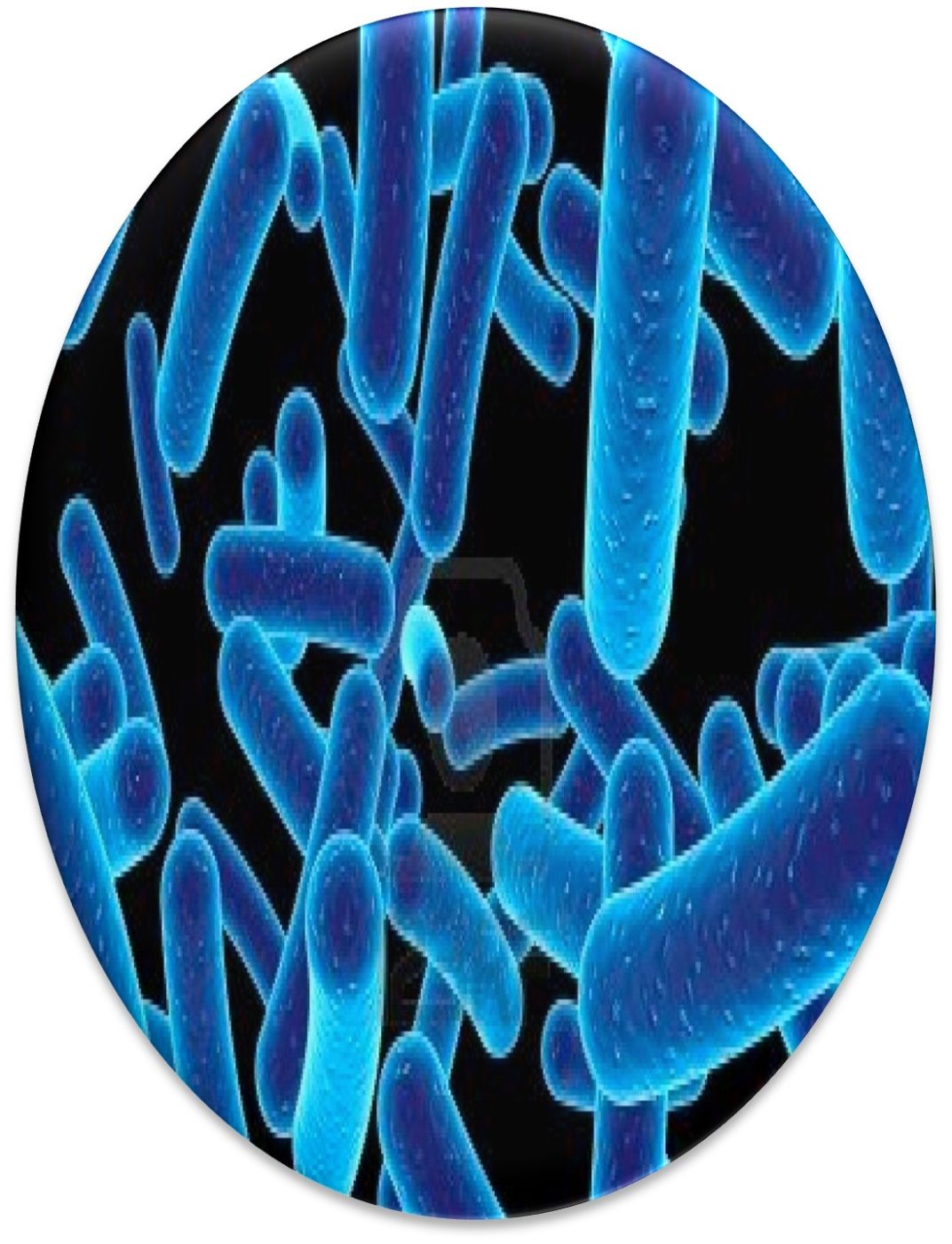
The Archaea were first discovered in thermal springs where the water temperature was nearly 100 °C (212 °F). Because their general shape (morphology) and size was like that of bacteria (Figure 2), and they lived in extreme environments that were thought to reflect those of Earth, more than 3 billion years ago, the Archaea were initially classified as “ancient” bacteria – Archaebacteria. Early investigators recognized that the isolates form extreme environments had some unique properties. They interpreted these properties as evidence that the Archaebacteria were the earliest forms of life. The logic was reasonable.
Archaea were (initially) only recovered from extreme environments that resembled early Earth, and
Archaea were apparently all chemolithotrophic or chemoheterotrophic anaerobes (see What’s New, 31 May 2023).
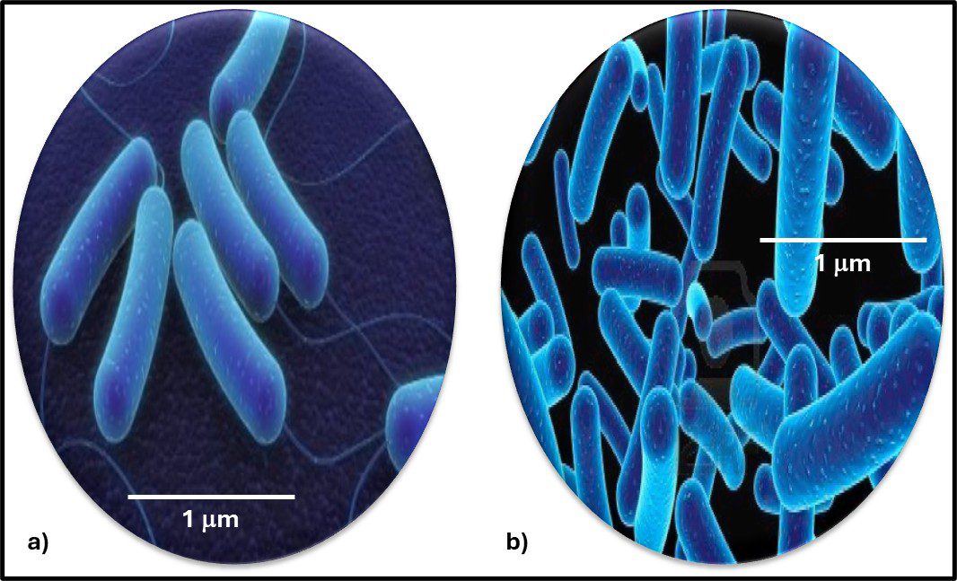
Fig 2. Prokaryotes – a) Archaea sp.; b) Bacteria (Pseudomonas sp.).
In time, both of these points turned out to be wrong.
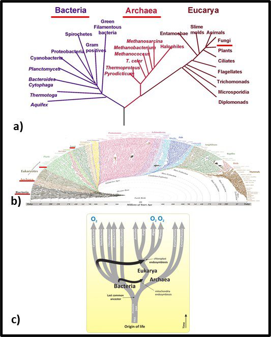
In 1977, Carl Woese and George E Fox at the University of Illinois at Champaign Urbana proposed a major revision to the tree of life. They postulated that genetic material – particularly ribonucleic acid (RNA) – could be used as an evolutionary clock. Differences in RNA from different organisms could be used to estimate when they split off from the last universal common ancestor (LUCA2). They also found that the RNA of Archaea was sufficiently different from that of bacteria to make the Archaea a kingdom of its own. Woese and Fox used the term Archaebacteria (from archaeon – ancient – and bacteria). As illustrated in Figure 3a, speculated that microbes in this kingdom were more ancient than the “true bacteria” (Eubacteria or Bacteria). Subsequent research has demonstrated that the Archaea are less ancient than the Bacteria (Figure 3b). In addition to their unique properties, they share some common characteristics with Bacteria and others with Eukaryotes.
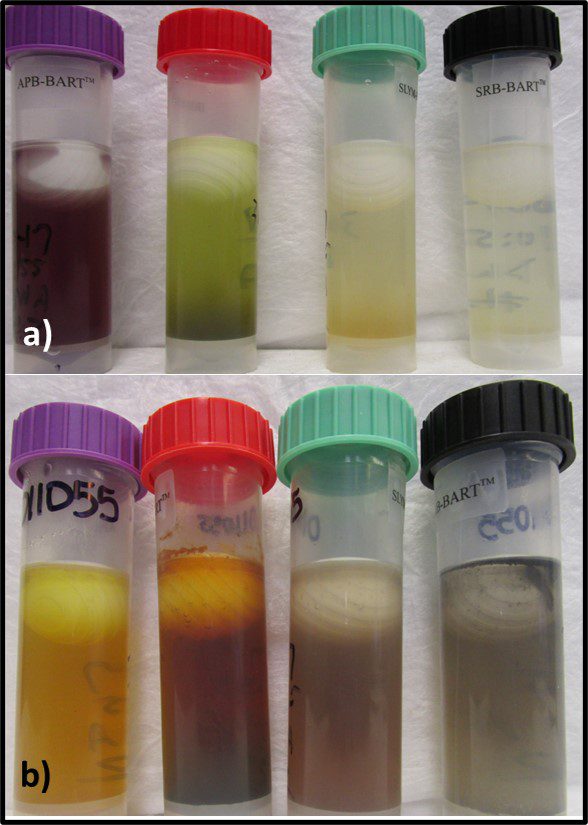
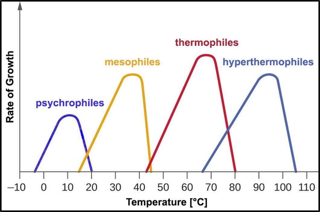
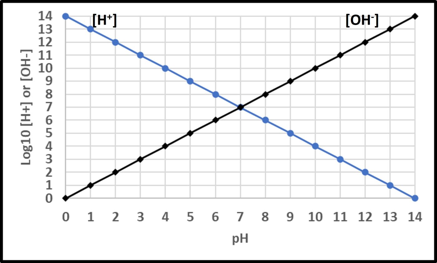
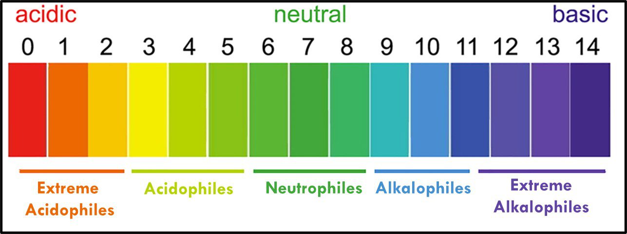
Archaea remain difficult to culture, although ~150 different Archaea taxa of the >2,000 taxa identified by metagenomics have now been grown in laboratories. Consequently, most of what is known about them has been determined by non-culture techniques. The original theory about all Archaea being extremophiles – requiring extreme environments such as high (>45 °C) or low temperature (<0 °C), salinity (brine), pressure (>10 kPa; 100 ATM), pH in the <1 or >11 range, or combinations of two or more of these conditions – reflected limited data rather than reality. Archaea have been recovered from many non-extreme environments; including industrial systems. Moreover, representatives of all of the physiological categories listed in Table 1 of my May 2023 What’s New post have been identified among the Archaea. Since they were first discovered in extreme environments, Archaea have been recovered in diverse ecosystems. They are as ubiquitous as bacteria.
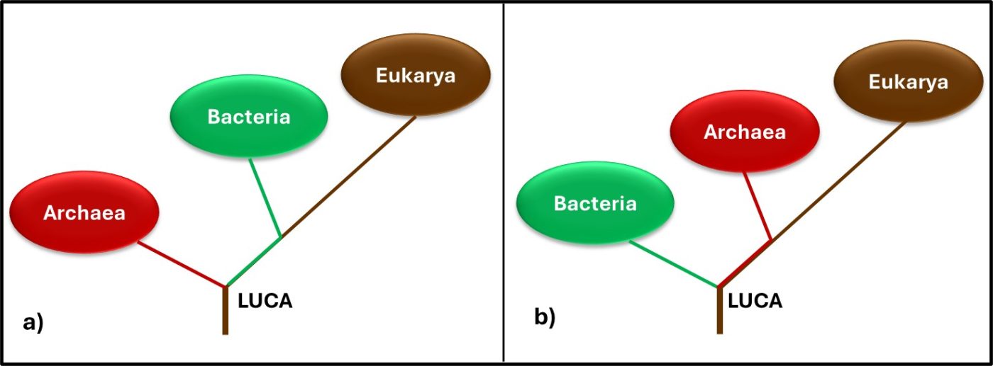
Fig 3. Two simplified phylogenic tree of life models – a) after Woese and Fox (1990); b) current model.
Archaea Phylogeny
Taxonomy and phylogeny are two approaches to categorizing organisms. Whereas taxonomy is based on the comparison of observable characteristics (plant versus animal, exoskeleton – shell – versus endoskeleton – bones; etc.), phylogeny attempts to categorize organisms based on their evolutionary relationships. Historically, biologists had no choice but to rely on taxonomy to classify organisms. The Woese and Fox evolutionary clock concept made it possible to rely on phylogenic methods (i.e., genomics) to classify organisms based on their genetic similarities. That said, in the arena of Archaeal phylogeny it is reasonable to paraphrase the words of former Secretary of State, Donald Rumsfeld, when he mentioned the unknown unknowns – those things we don’t know that we don’t know. Figure 4 illustrates a recent phylogenic tree for Archaea, but the model is not universally accepted and is likely to continue to be modified as researchers learn more about the Archaea. Note that the lengths of the lines and points where lines branch off in Figure 4 reflect genetic relationships among the different taxa.
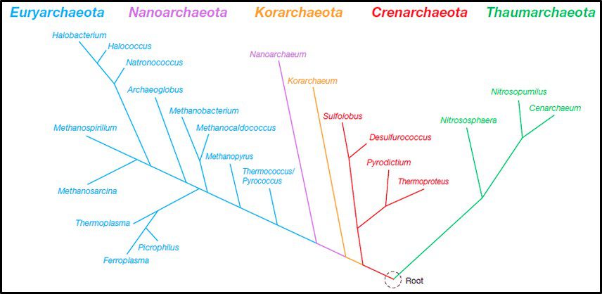
Fig 4. Phylogenic tree of Domain Archaea depicting five phyla (Source: https://www.researchgate.net/publication/274708754_Archaea_Morphology_Physiology_Biochemistry_and_Applications)
The phylum Euryarchaeota includes methanogens (Archaea able to produce methane form hydrogen and carbon dioxide or acetate), halophilic taxa (Archaea that thrive in saturated salt brine), and some extreme thermophiles (some of which grow at >120 °C – >248 °F). Thus far Nanoarchaeota includes only one species – Nanoarchaeum equitans – an organism that was discovered near a deep-sea thermal vent. N. equitans is nominally spherical, and as its name implies, is <0.6 μm diameter. Similarly, the Korarchaeota thus far includes only a single genus of extremely thermophilic archaea. Crenarchaeota were initially recovered from thermal springs and thought to be acidophilic (thriving in pH 2 to 4 water), thermophilic organisms. Subsequently Crenarchaeota genera were discovered to be ubiquitous in marine sediments and freshwater environments. In 2005, an ammonia oxidizing species was recovered from a marine aquarium tank. The Thaumarchaeota (AKA Nitrososphaerota) primarily includes ammonia oxidizers.
Archaeal Cell Morphology
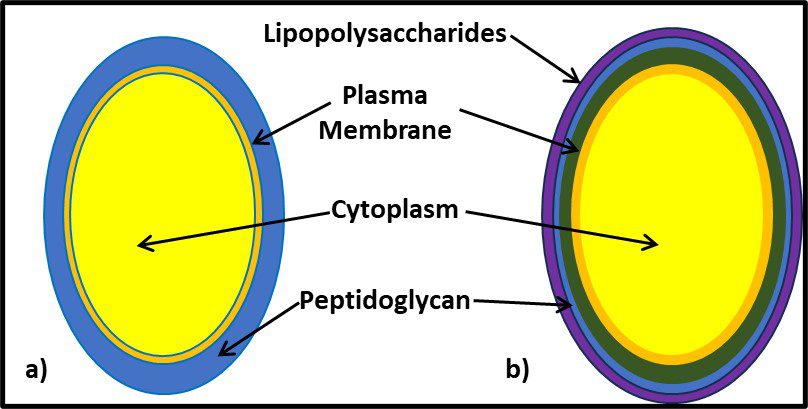
One distinguishing feature of archaeal cells is their unique cell wall and membrane chemistries. As illustrated in Figure 5, unlike bacterial and eukaryotic cell membranes that are comprised of D-glycerol, ester-linked lipids, archaeal cell membranes have branched tailed, ether-linked, L-glycerol lipids. Archaeal cell walls are comprised of S-layer proteins or pseudopeptidoglycan (N-acetylglucosamine and N-acetyltalosaminuronic acid) or S-layer proteins, but no peptidoglycan. All bacterial cell walls have a peptidoglycan layer (Figure 6).
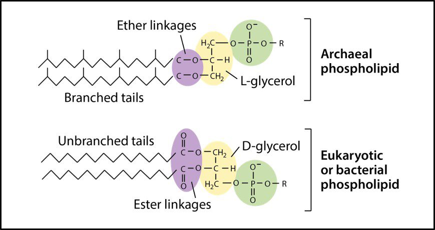
Fig 5. Schematic drawings of Archaeal cell membrane phospholipids (top) and those of bacteria and Eukaryotes (Source: https://cdn.kastatic.org/ka-perseus-images/9d44a501fb30b8301640773ed409226119208fdf.png).
Morphologically, the Archaea are quite diverse. Their size ranges from <1 μm to >150 μm. Their geometry can be spherical, obround, or spiraled. Some methanogens are disk-shaped and some thermophiles have irregular shapes (Figure 7).
Comparing Archaea and Bacteria
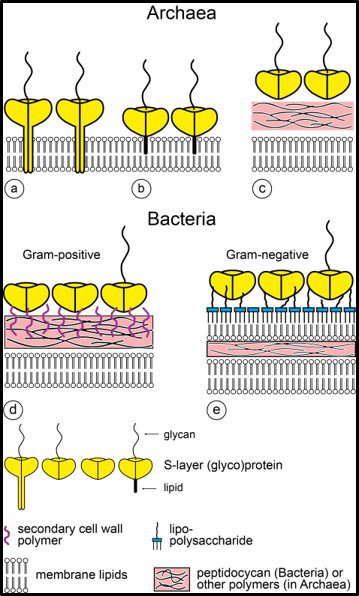
Fig 6. Schematic illustration of the supramolecular architecture of the major classes of prokaryotic cell envelopes containing surface (S) layers. S-layers in archaea with glycoprotein lattices as exclusive wall component are composed either of mushroom-like subunits with pillar-like, hydrophobic trans-membrane domains (a), or lipid-modified glycoprotein subunits (b). Individual S-layers can be composed of glycoproteins possessing both types of membrane anchoring mechanisms. Few archaea possess a rigid wall layer (e.g. pseudomurein in methanogenic organisms) as intermediate layer between the plasma membrane and the S-layer (c). In Gram-positive bacteria (d) the S-layer glycoproteins are bound to the rigid peptidoglycan-containing layer via secondary cell wall polymers. In Gram-negative bacteria € the S-layer is closely associated with the lipopolysaccharide of the outer membrane (Source: Sleytr UB, et al. (2014). “S-layers: Principles and Applications”. FEMS Microbiology Reviews. 38 (5): 823–864. doi:10.1111/1574-6976.12063).
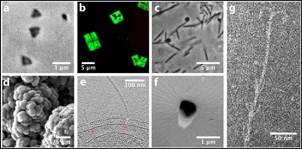
Fig 7. Diversity of Archaeal cell morphologies – a) Brightfield image of the triangular-shaped Haloarcula japonica cells; b – The square and flat Haloquadratum walsbyi cells with DNA stained with acridine orange; c – contrast-phase of rods and “golf clubs” cells of Thermoproteus tenax; d – Scanning electron micrograph image of multicellular clusters of the coccoid Methanosarcina spp. Culture from environmental samples; e – Cryoelectron tomograph of a Thermococcus kodakaraensis cell showing a conical basal body (bottom structure) anchoring the archaellum (top structure) to the cytoplasm; f – Electron micrograph of the cold-living SM1 euryarchaeon showing several pili-like hami fibers around the entire cell surface; g – Electron micrograph of a section of a filamentous hamus showing its hook (tip) and prickle (body) structures (Source: Bisson-Filho et al. (2018), https://doi.org/10.1091/mbc.E17-10-0603).
Table 1 summarizes other similarities and differences between Archaea and Bacteria. Archaea also share characteristics with Eukaryotes.
Table 1. Comparisons between Archaea and Bacteria
| Property | Archaea | Bacteria |
|---|---|---|
| Cell type | Prokaryote | Prokaryote |
| Cellular organization | Single cell (unicellular) | Single cell |
| Cell organelles | No membrane-bound internal structures (organelles) | No membrane-bound internal structures |
| Chromosomes | Circular (like Bacteria); transcription & translation like Eukaryotes | Circular; unique transcription & translation |
| Horizontal gene transfer (HGT) | Many taxa exhibit HGT | HGT is rare |
| Histone and histone-like proteins | Present | Absent |
| Intronsa | Present (also in Eukaryotes) | Absent |
| Ribosomal RNA (rRNA) | rRNA sequences unique to Archaea | rRNA sequences different than for Archaea |
| Reproduction | Fission (asexual) | Fission |
| RNA polymerase enzymes | Multiple & complex (like Eukaryotes) | Single enzyme |
Ecological Significance
Based on their ubiquity and metabolic diversity in terms of energy metabolism (autotrophy – using carbon dioxide as their energy source, chemolithotrophy – using ammonia, sulfide, or other inorganic molecules as their energy source, photolithotropy – obtaining energy from sunlight) Archaea play important roles in carbon, nitrogen, and sulfur biogeochemical cycles (biogeochemical cycles are the natural processes by which nutrient elements move between organisms and the environment – I’ll discuss biogeochemical cycles in the next several What’s New articles). Methanogenesis plays an important role in anaerobic sewage sludge digestion. Methane captured from digesters and landfills is used for power generation and in gas-powered vehicles. Recent research has suggested that Archaea comprise >20 % of the total biomass in marine environments. Again, they play critical roles in biogeochemical cycling in marine sediments. It is likely that they play similar roles in other aquatic ecosystems.
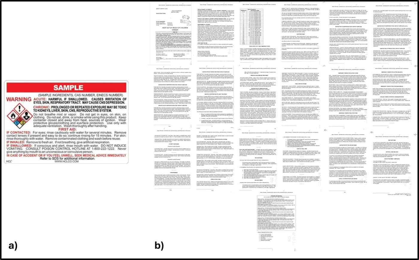
Are Archaea Biodeteriogenic?
Earlier, I paraphrased the third part of Secretary Rumsfeld’s “unknowns” quote. The answer to the question of whether Archaea are biodeteriogenic evokes the second part of the quote: “There are known unknowns. That is to say there are things we now know that we do not know.” For most of the history of microbiological contamination condition monitoring, the primary tool has been culture testing. As with every other tool for detecting and quantifying microbiological contamination, culture testing has benefits and limitations. Recognizing that nutrient media and incubation conditions routinely used for routine culture testing do not detect Archaea, until recently, Archaea have remained undetected in industrial systems. Archaea abundance, distribution, and metabolic activities in industrial systems remain known unknowns. Until recently, the cost of genomic testing was prohibitive for routine condition monitoring. As commercially available test kits at relatively modest cost have become available the potential to learn about whether or how Archaea contribute to biodeterioration has become feasible. The presence of Archaea in petroleum formations has been well documented. To date, there have been only a few reports of Archaea in fuels, metalworking fluids, and other industrial systems. Consequently, although it is reasonable to speculate that Archaea play a role in biodeterioration, there is no concrete evidence to support that speculation. In the flip side, a growing number of researchers are investigating the use of Archaea in fuel cells.
Summary
The Archaea were identified as a unique biological domain only 45 years ago. Initially, their distribution in nature was believed to be restricted to extreme environments such as hot springs, acid mine drainage streams, and salt evaporation ponds. Their ubiquitous distribution and essential role in nutrient cycling has only been recognized in the past two decades. The tools for detecting Archaea as part of routine condition monitoring programs are only now becoming available. Industries in which microbiology expertise is rare and reliance on the oldest test methods is the norm are unlikely to develop substantial data on Archaea distribution or abundance. Consequently, much remains to be learned about whether or how Archaea contribute to biodeterioration.
As always, please share your comments and questions with me at fredp@biodeterioration-control.com.
1 Árbol de la vida según Haeckel, E. H. P. A. (1866).Generelle Morphologie der Organismen : allgemeine Grundzüge der organischen Formen-Wissenschaft, mechanisch begründet durch die von C. Darwin reformirte Decendenz-Theorie. Berlin.
2 Weiss, Madeline C.; Sousa, F. L.; Mrnjavac, N.; et al. (2016). “The physiology and habitat of the last universal common ancestor” (PDF). Nature Microbiology. 1 (9): 16116.