FUEL & FUEL SYSTEM MICROBIOLOGY PART 8 – CHOOSING TEST METHODS B

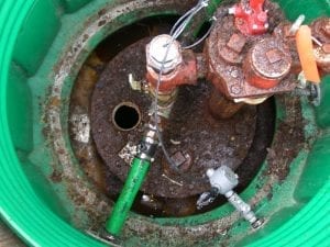
STP spill containment well.  Good news: well has a 4 inch port for testing bottoms-water height and collecting bottoms samples.  Bad News: there is lots of corrosion.

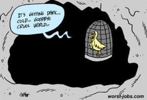
The canary in the coal mine….

In my last post, I discussed the kinds of questions that should be asked before deciding on what tests to run and how frequently to run them.  Now I’ll share my condition monitoring (CM) philosophy with you. I’ll list them as axioms – statements that should seem obvious to the most casual of observers. 

Axiom 1: For most frequent testing, rely on methods that are easy to perform and interpret.  The flow-rate example that I shared in Part 7 (16 February 2017) illustrates this point.  You can test dispenser flow-rate while filling your vehicle.  The only test equipment you need is a stop watch, or flow-rate APP (I don’t want to be commercial here, but I know of at least one fuel system service company that offers a free, dispenser flow-rate APP). 

Axiom 2: The tests you run most frequently should be your canaries in the coal mine¹.  I call these simple, frequently run tests 1^st Tier tests.  They don’t tell you much about why there is a problem, but signal either that a problem exists, or that the risk of a problem developing has increased.  Examples of other 1^st Tier tests include:

• Bottoms-water detection, by water-paste on fuel gauging stick or sounding bob.
• Standing water in spill containment wells.
• Broken spill containment well covers.
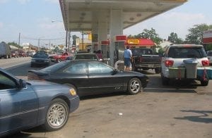
• Heavily corroded submerged turbine pump (STP), turbine distribution manifold (see photo above).

The common feature of these tests is that they require very little technical training or test equipment.

Axiom 3 (repeat from Part 7): Every parameter that you test must have control limits! You need to know what is normal and what isn’t.  I like the green, amber, and red light approach. 

• When conditions are normal, you have a green light.
• When conditions are not quite normal, but operations don’t seem to be affected, you are in the amber light zone. This is the time to run additional tests or schedule preventive/early corrective maintenance. This is the zone that links CM to predictive maintenance (PdM – see Part 5).
• The red-light zone indicates that you are having problems. You need to schedule corrective maintenance as soon as possible. When your site has a well-planned, well executed CM program, you never get red zone test results. Red-light results signal both operational and PdM program problems.

Axiom 4: 1^st Tier, amber-light results should trigger either maintenance actions or 2^nd Tier tests.

• Action example: if you detect water in a spill containment well or tank bottom, remove it. There’s no need for additional testing to help you determine the best course of action.
• 2^nd Tier testing example: If your dispenser flow-rate <80% of maximum, use 2^nd Tier testing to determine why.  Remember: slow-flow is not the same as a plugged filter!  There are several chokepoints (for example: screens) between the STP and dispenser nozzle.  Moreover, slow-flow after a 500 000 gal of fuel have passed through a dispenser filter tells a much different story than slow-flow after 50 000 gal have been filtered (see the flow-rate testing example in Part 7).

Axiom 5: 2^nd Tier tests should be diagnostic, but sufficiently easy to perform so that a trained technician can complete the testing on-site. In most cases, 2^nd Tier test results provide sufficient information to guide maintenance actions.  I break 2^nd Tier tests into four categories, and will discuss each category in more detail in the next four MICROBIAL DAMAGE blog posts. I list the categories here:

• Gross observations
• Physical tests
• Chemical tests
• Microbiological tests

There are rare occasions when the 2^nd Tier test results are inconclusive.  Additional testing is needed to diagnose what’s going on.  In most cases, 3^rd Tier tests are run at specialty testing labs.  These are labs that have particular expertise in fuel, corrosion, or microbiological testing.  Examples of 3^rd Tier testing include:

• Corrosion deposit analysis
• Fuel property testing (this typically includes tests listed in ASTM fuel specifications)
• Bottoms-water chemistry testing
• Fuel or bottoms-water microbiology testing (detailed tests to determine the types of microbes present)

One very rare occasions, 4^th Tier or 5^th Tier tests are run to gain a deeper understanding of the processes that increase operational risks.  These higher tier tests are typically run as part of research efforts rather than in direct support of troubleshooting.  There is still quite a bit that we do not know about what causes fuel quality problems and fuel system failures.

As I have noted in previous posts in this series, in each post, I’m peeling back another layer of a complex onion.  If you are impatient and want to learn more now, don’t hesitate to contact me at fredp@biodeterioraiton-control.com. 

¹ In the days before electronic oxygen and explosive gas detectors, miners would use canaries as hazard alarms.  If methane or carbon dioxide concentrations became too high, the canaries would die.  The canaries’ sudden silence would alert miners that they needed to evacuate the mine – high methane meant high explosion risk! (more…)

FUEL & FUEL SYSTEM MICROBIOLOGY PART 7 – CHOOSING TEST METHODS A

How do we select condition monitoring tests?

Parts 3 and 4 of this series introduced the issue of test method selection. Starting with Part 7, I’ll spend the next few posts drilling down into different testing options when you want to evaluate fuel system microbiological contamination.
Today let’s start with two questions. These are the two questions that should drive most predictive maintenance test decisions:
→What do I need to know to be sure I have a microbial contamination problem?
→What will I do with test results?
Although microbiology data are useful – even important – they are only part of the story. This means that the first question’s answer is not necessarily microbiology data. In this blog post, I’ll focus on the first question.

What do I need to know to be sure I have a microbial contamination problem?
There’s an old joke in which one person asks another: “Why do you always answer my questions with a question?”. The person to whom the question was posed responds: “Do I?” In the same vein, the answer to What do I need to know? is What will you do with the results? There is no benefit to running any test if the results do not drive some action when the results indicate that conditions are not normal (i.e.: in specification). This means that when a technician is tasked with running a test, they need to know three things:
       • How to run the test
       • What the test results indicate
       • The next action to be taken if the results indicate that conditions are not normal.
Running tests – every test method should be detailed in a standard operating procedure (SOP) document. This SOP can be an ASTM, PEI or other method developed as a consensus standard. It can be a method developed by an employer. As I noted in Part 5, the Navy uses Maintenance Requirement Cards (MRC). A well written SOP lists all materials, supplies and tools needed to perform the task. It lists both hazards and potential interferences. It then provides detailed instructions for how to complete the task. Next, test method SOP specify what to report and how to report the results plus supporting information. Finally, the test method SOP provides guidance on how to interpret the results and what action to take.
What the results indicate – some methods generate numerical data. For example, one of the easiest tests to run is dispenser flow-rate. The technician either determines how long it takes to dispense a specified volume of fuel, or determines how much fuel is dispensed during a fixed time. The results are reported as gallons (or liters) per minute (gpm). Without some context, the results are not particularly helpful. However, we can assign attribute scores to flow-rate ranges; for example:
       • 8 gpm ((30 l/min) to 10 gpm (38 l/min): normal;
       • 6 (23 l/min) gpm to <8 gpm: moderately reduced; and
       •<6 gpm: severely reduced.  For fleet operations, the breakpoints might be 36 gpm (136 l/min) and 24 gpm (91 l/min). 

Having assigned attribute scores to our raw data, we know that the flow-rate of a retail dispenser dispensing fuel at 4 gpm (15 l/min) is severely reduced. Some action is needed.

What action is needed? – most often – particularly for quick and dirty tests – the action triggered by a test result that indicates that there is a problem, is additional testing. In our dispenser flow-rate example, the severely reduced flow can be a symptom of different causes; including microbiological contamination.

For example, if the test is run when several dispensers are being operated, the pump might not have sufficient power to deliver full flow to all active dispensers. An under-capacity pump has nothing to do with microbiological contamination. Alternatively, reduced flow could be a symptom of contamination. Again, not all contamination is microbial. Moreover, the assumption that slow-flow is due to filter plugging can be wrong. This leads to a set of IF/THEN instructions:

     • IF flow <6 gpm, THEN retest after confirming that no other dispensers are operating.
     • IF flow <6 gpm when no other dispensers are operating, THEN replace filter and retest flow rate.
     • IF flow is <8 gpm after replacing filter; THEN clean dispenser prefilter (screen) and retest flow rate.
     • IF flow rate is <8 gpm after cleaning prefilter; THEN test leak detector, replace if necessary, and retest flow rate.
     • IF flow rate <8 gpm after testing/replacing leak detector; THEN test/repair/replace submerged turbine pump and retest flow rate.

Notice that in each case, the level of effort is greater and the flow rate is retested after the action has been completed.
By now, perhaps you are wondering: All this is interesting but what do I really need to know to be sure I have a microbial contamination problem? Stay tuned. In Part 8, I’ll offer some approaches to how you can answer that question.

Flow-rate testing as I’ve described here is one example of tiered testing. Here I reran the same test after taking increasingly complex maintenance actions. In future posts, I’ll write about more tiered testing in which the results from a simple test trigger the need to run a more complex test. I’ll also discuss individual test methods and share my opinions about their respective advantages and limitations. If you are impatient and want to learn more now, contact me at fredp@biodeterioraiton-control.com.