
The tool you choose depends on the intended use.
A Bit More About Relative Bias
In my last post I introduced the concept of relative bias. I wrote that unless there is a reference standard against which a measurement can be compared, only relative bias – the difference between test results obtained by different methods – can be assessed. In my example, I compared the results of two test methods for determining the concentration of end-use diluted metalworking fluids (MWF). Before moving on to comparisons among methods that measure different properties, I’ll share another illustration to show how relative bias differs from bias. In figures 1 a & 1b (figure 1 in July’s What’s New article) bias can be measured as the distance between the average value of the respective data clusters (yellow dots) and the bullseye’s center. However, in figure 1c, there is no target or bullseye – no reference point against which to assess the two data sets for their respective biases. In situations like this, we can only calculate the direction and magnitude between the two data clusters – the relative bias between the two methods. We cannot use these data to assess which method is more accurate.

Comparing Two Different Parameters
Culture test fundamentals
Figure 2 from my July 2017 article illustrates the basic principle of culture testing. A nutrient medium is inoculated with a specimen and incubated under a standard set of conditions (i.e., temperature and atmosphere). Those microbes that can use the nutrients provided, under the incubation conditions used (for example, aerobic bacteria require oxygen, but anaerobic bacteria will not proliferate – multiply – unless the atmosphere is oxygen-free) will reproduce. Generation time is the period that lapses between cell divisions. For most known bacteria, generation times range from ∼15 min to ∼8 h. Typically, colonies (cell masses) become visible only after ∼109 (1 billion) cells have accumulated. This equals 30 generations (230). Thus, the time needed for a single cell to produce a visible colony can vary from 7.5 h ((30 generations x 0.25 h/generation) to 10 days (30 generations x 8 h/generation = 240 h = 10 d). Microbes that cannot proliferate under the test’s conditions remain undetected. Additionally, in specimens with microbes that have a range of generation times, the colonies of microbes with longer generation times are likely to be eclipsed by those of microbes with shorter generation times (figure 3). These two factors contribute to bioburden underestimations.


Chemical test fundamentals
Chemical tests include a variety of methods that detect specific microbial molecules. For example, quantitative polymerase chain reaction (qPCR) test methods detect the number of copies of specific genes. The results are reported as gene copies per mL (GC mL-1). Adenosine triphosphate (ATP) tests measure the number of photons of light emitted by the reaction of the enzyme luciferase with the substrate luciferin (see What’s New, August 2017 We know that organisms typically have multiple copies of various genes, and that the number of copies of a given gene varies among microbes with that gene. Similarly, we know that the number of ATP molecules varies among types of microbes (figure 4a) and organisms’ physiological states (figure 4b). Despite this, both qPCR and ATP data generally agree with culture test data and other chemical tests for bioburden.

Although the [cATP] per bacterial cell is nominally 1 fg cell-1 (1 x 10-15 g cell-1), it can vary from 0.1 fg cell-1 to 50 fg cell-1, depending on the bacterial species present and whether they are healthy or stressed. I find it quite remarkable that despite the [cATP] per cell range, >60-years of studies on ATP-bioburden support the use of 1 fg cell-1 as a suitable basis for estimating ATP-bioburdens in many different types of samples.
Correlation coefficients
When comparing two different microbiological test methods such as culturability (CFU mL-1) and ATP-bioburden ([cATP] pg mL-1), we are interested in correlation (i.e., the correlation coefficient (r)) or agreement.
In last month’s What’s New article, I introduced the concept of correlation coefficient. The correlation coefficient (r) is the most common statistical tool for determining the relationship between two parameters. The value, r, can range from -1.0 to +1.0. The closer r comes to either +1.0 or -1.0, the stronger the relationship between the two parameters. If r’s sign is negative one parameter’s value increases as the other’s decreases. This is called a negative or inverse correlation. In Comparing Microbiological Test Methods – Part 1, figure 5 illustrated the relationship between two test methods used to determine water-miscible metalworking fluid concentration ([MWF]) at various end-use dilutions. The slope of the correlation curve ≈1 and r = 1.0 – indicating that for the MWF tested, the results obtained by acid split and refractometer reading agreed perfectly at the 95 % confidence level.
Contrast that plot with figure 5, below – a series of 10-fold dilutions of a sample that has 5.5 Log10 CFU mL-1 (3.2 x 10⁵ CFU mL-1) you should get a regression curve that looks like the one in figure 5 (July’s figure 5). In this graph r ≈ -1.0 – showing an inverse relationship between dilution factor and CFU mL-1.

When r = 0, there is no relationship between the parameters. Figure 6 is a plot of CFU mL-1 versus sample volume. In this example, r = 0.022 ≈ 0. As expected, CFU mL-1 values do not vary with sample volume.

The critical value of r is the value at or above which the relationship between two parameters is statistically significant at a predetermined confidence level. The most commonly used confidence level is 95 % (α = 0.05). This means that there is a 5 % chance that a correlation will be interpreted as being statistically significant, when it isn’t (in statistics, this is known as a type I error).
The minimum value of r that is considered to be statistically significant (rcrit; α = 0.05) decreases as the number of samples tested (n) increases. For example, when n = 10, rcrit; α = 0.05 = 0.63, but when n = 100, rcrit; α = 0.05 = 0.20.
An assessment of the strength of the correlation between two parameters depends on what you are measuring. In many fields, correlations are categorized as strong, moderate, weak, or non-existent. However, the thresholds vary. Without consideration of the value of n, the categories can be misleading. That said, in general r > 0.75 is typically considered to indicate a strong relationship. Moderate relationships are indicated when 0.50 < r ≤ 0.75, and weak relationships are indicated when 0.25 < r ≤ 0.50. As used here, the terms strong, moderate, and weak are categorical – they identify categories of r-values.
Agreement between methods – attribute scores
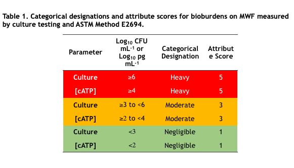
In industrial process control microbial bioburdens are typically classified into two or three categories based on control limits. For example, in MWF systems, culturable bioburdens <103 CFU mL-1 (<3Log10 CFU mL-1) are considered negligible, ≥103 CFU mL-1 to <106CFU mL-1 are moderate, and ≥106 CFU mL-1 are heavy. Negligible, moderate, and heavy are categorical designations. To facilitate computations, categorical designations are typically assigned numerical values – attribute scores. Table 1 lists the categorical designations and attribute scores for culture test and ASTM E2694 cellular ATP [cATP] in water-miscible MWF. Note that assignment to categories is a risk management decision that reflects the need to strike a balance between costs associated with microbial contamination control and those associated with fluid failure. That’s a topic for a future What’s New article.
In my next article – Comparing Microbiological Methods – Part 3 – I’ll apply the concepts I’ve explained in this article to actual test method comparisons.
I look forward to receiving your questions and comments at fredp@biodeterioration-control.com.
