
The Confusion
Over the past several months, I have received questions about the impact of test method sensitivity on control limits. In this post, I will do my best to explain why test method sensitivity and control limits are only indirectly related.
Definitions (all quotes are from ASTM’s online dictionary)
Accuracy – “a measure of the degree of conformity of a value generated by a specific procedure to the assumed or accepted true value and includes both precision and bias.”
Bias – “the persistent positive or negative deviation of the method average value from the assumed or accepted true value.”
Precision – “the degree of agreement of repeated measurements of the same parameter expressed quantitatively as the standard deviation computed from the results of a series of controlled determinations.”
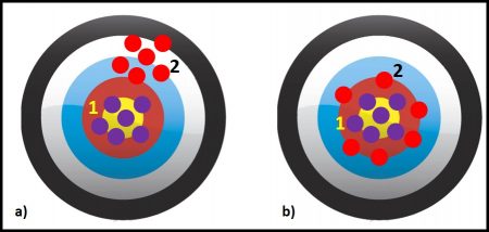
Figures 1a and b illustrate these three concepts. Assume that each dot is a test result. The purple dots are results from Method 1 and the red dots are from Method 2. In figure 1a, the methods are equally precise – the spacing between the five red dots and between the five purple dots is the same. If these were actual measurements and we computed the average (AVG) values and standard deviations (s), s1 = s2. However, Method 1 is more accurate than Method 2 – the purple dots are clustered around the bull’s eye (the accepted true value) but the red dots are in the upper right-hand corner, away from the bull’s eye. The distance between the center of the cluster of red dots and the target’s center is Method 2’s bias.
Limit of Detection (LOD) – “numerical value, expressed in physical units or proportion, intended to represent the lowest level of reliable detection (a level which can be discriminated from zero with high probability while simultaneously allowing high probability of non-detection when blank samples are measured.” Typically test methods have a certain amount of background noise – non-zero instrument readings observed when the test is run on blanks (test specimens known to have none of the stuff being analyzed).
I have illustrated this in figures 2a through c. Figure 2a is a plot of the measured concentration (in mg kg-1) of a substance being analyzed (i.e., the anylate) by Test Method X. When ten blank samples (i.e., anylate-free) are tested, we get a background reading of 45 ± 4.1 mg kg-1. The LOD is set at three standard deviations (3s) above the average background reading. For test Method X, the average value is 45 mg kg-1 and the standard deviation (s) is 4.1 mg kg-1. The average + 3s = 57 mg kg-1. This means that, for specimens with unknown concentrations of the anylate, any test results <57 mg kg-1 would be reported as below the detection limit (BDL).
Now we will consider Test Method Y (figure 2b). This method yields background readings in the 4.1 mg kg-1 to 5.2 mg kg-1 range. The background readings are 4.4 ± 0.4 mg kg-1 and the LOD = 6 mg kg-1. Figure 2c shows the LODs of both methods. Because Method Y’s LOD is 48 mg kg-1 less than Method X’s LOD, it is rated as a more sensitive – i.e., it can provide reliable data at lower concentrations.
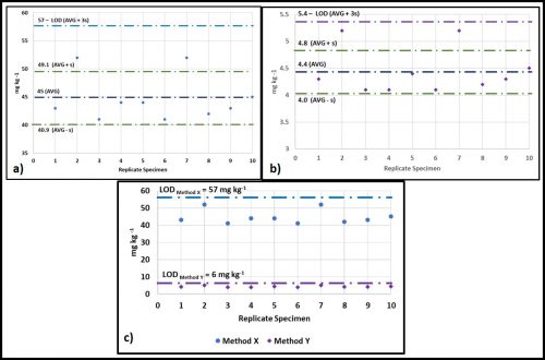
Limit of Quantification (LOQ) – “the lowest concentration at which the instrument can measure reliably with a defined error and confidence level.” Typically, the LOQ is defined as 10 x LOD. In the figure 1 example, Test Method X’s LOQ = 10 x 57 mg kg-1, or 570 mg kg-1, and Test Method Y’s LOQ = 10 x 6 mg kg-1, or 60 mg kg-1.
Type I Error – “a statement that a substance is present when it is not.” This type of error is often referred to as a false positive.
Type II Error – “a statement that a substance was not present (was not found) when the substance was present.” This type of error is often referred to as a false negative.
Control limits – “limits on a control chart that are used as criteria for signaling the need for action or for judging whether a set of data does or does not indicate a state of statistical control.”
Upper control limit (UCL) – “maximum value of the control chart statistic that indicates statistical control.”
Lower control limit (LCL) – “minimum value of the control chart statistic that indicates statistical control.”
Condition monitoring (CM) – “the recording and analyzing of data relating to the condition of equipment or machinery for the purpose of predictive maintenance or optimization of performance.” Actually, this CM definition also applies to condition of fluids (for example metalworking fluid concentration, lubricant viscosity, or contaminant concentrations).
Why worry about LOD & LOQ?
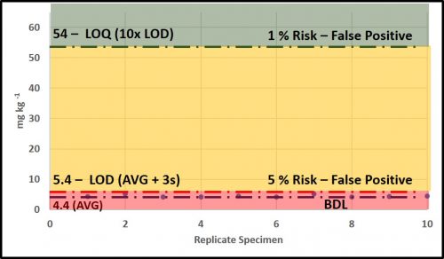
Taking measurements is integral to condition monitoring. As I will discuss below, we use those measurements to determine whether maintenance actions are needed. If we commit a Type I error and conclude that an action is needed when it is not, then we lose productivity and spend money unnecessarily. Conversely, if we commit a Type II error and conclude no action is needed, although it actually is, we risk failures and their associated costs. Figure 3 (same data as in figure 2c) illustrates the risks associated with data at the LOD and LOQ, respectively. Measurements at the LOD (6 mg kg-1) have a 5 % risk of being false positives (i.e., one measurement out every 20 is likely to be a false positive). At the LOQ (60 mg kg-1) the risk of obtaining a false positive is 1 % (i.e., one measurement out every 100 is likely to be a false positive). As illustrated in figure 3, in the range between LOD and LOQ, test result reliability improves as values approach the LOQ.
The most reliable data are those with values ≥LOQ. Common specification criteria and condition monitoring control limit for contaminants have no lower control limit (LCL). Frequently operators will record values that are LOD as zero (i.e., 0 mg kg-1). This is incorrect. These values should be recorded either as “LOD” – with the LOD noted somewhere on the chart or table – or as “X mg kg-1” – where X is the LOD’s value (6 mg kg-1 in our figure 3 example). In systems that are operating well, analyte data will mostly be LOD and few will be >LOQ. For data that fall between LOD and LOQ, a notation should be made to indicate that the results are estimates.
Take home lesson – accuracy, precision, bias, LOD, and LOQ are all characteristics of a test method. They should be considered when defining control limits, but only to ensure that control limits do not expect data that the method cannot provide. More on this concept below.
Control Limits
Per the definition provided above, control limits are driven by system performance requirements. For example, if two moving parts need at least 1 cm space between them, the control limit for space between parts will be set at ≥1 cm. The test method used to measure the space can be a ruler accurate to ±1 mm (±0.1 cm) or a micrometer accurate to 10 μm (0.001 cm), but should not be a device that is cannot measure with ±1 cm precision.
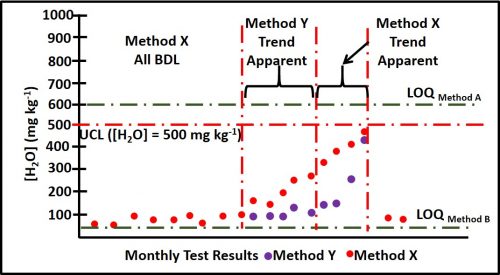
Control limits for a given parameter are determined based on the effect that changes in that parameter’s values have on system operations. Referring back to figures 2a and b, assume that the parameter is water content in fuel and that for a particular fuel grade, the control objective was to keep the water concentration ([H2O]) < 500 mg kg-1. Method X’s LOD and LOQ are 57 mg kg-1 and 570 mg kg-1, respectively. Method Y’s LOD and LOQ are 5.4 mg kg-1 and 54 mg kg-1, respectively. Although both methods will detect 500 mg kg-1, under most conditions, Method Y is the preferred protocol.
Figure 4 illustrates the reason for this. Imagine that Methods X & Y are two test methods for determining total water in fuel. [H2O] = 500 mg kg-1 is near, but less than Method X’s LOQ. This means that whenever water is detected a maintenance action will be triggered. In contrast, because [H2O] = 500 mg kg-1 is 10x Method Y’s LOQ, a considerable amount of predictive data can be obtained while [H2O] is between 54 mg kg-1 and 500 mg kg-1. Method Y data detects an unequivocal trend of increased [H2O] five months before [H2O] reaches its 500 mg kg-1 UCL and four months earlier than Method X detects the trend.
Note that the control limit for [H2O] is based on risk to the fuel and fuel system, not the test methods’ respective capabilities. Method Y’s increased sensitivity does not affect the control limit.
A number of factors must be considered before setting control limits. I will address them in more detail in a future blog. In this blog I will use jet fuel microbiological control limits to illustrate my point.
Historically the only method available was culture testing (see Fuel and Fuel System Microbiology Part 12 – July 2017 Fuel and Fuel System Microbiology Part 12 – July 2017). The UCL for negligible growth was set at 4 CFU mL-1 (4,000 CFU L-1) in fuel and 1,000 CFU mL-1 in fuel associated water. By Method ASTM D7978 (0.1 to 0.5 mL fuel is placed into a nutrient medium in a vial and incubated) 4,000 CFU L-1 = 8 colonies visible in the vial after incubating a 0.5 mL specimen. For colony counts the LOQ = 20 CFU visible in a nutrient medium vial (i.e., 40,000 CFU L-1). As non-culture methods were developed and standardized (ASTM D7463 and D7687 for adenosine triphosphate; ASTM D8070 for antigens), the UCLs were set, based on the correlation between the non-culture method and culture test results.
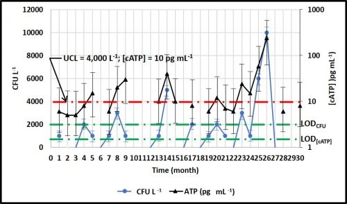
Figure 5 compares monthly data for culture (ASTM D7978) and ATP (ASTM D7687) in fuel samples. The ASTM D7979 LOD and LOQ are provided above. The ASTM D7687 LOD and LOQ are is 1 pg mL-1 and 5 pg mL-1, respectively. The figure 5, green dashed lines show the respective LOD. The D7978 and D7687 action limits (i.e., UCL) between negligible and moderate contamination are 4,000 CFU L-1 and 10 pg mL-1, respectively (figure 5, red dashed line). The figure illustrates that over the course of 30 months, none of the culture data were ≥LOQCFU . In contrast, 22 ATP data points were ≥LOQ[cATP] and five occasions, D7687 detected bioburdens >UCL when D7978 data indicated that CFU L-1 were either BDL or UCL.
Additionally, as illustrated by the black error bars in figure 5, the difference of ±1 colony in a D7978 vial has a substantial effect on the results. For the 11 results that were >BDL, but <4,000 CFU L-1, the error bars indicate a substantial Type II error risk – i.e., assigning a negligible score when the culturable bioburden was actually >UCL. Because D7687 is a more sensitive test, the risk of making a Type II error is much lower. Moreover, because there is a considerable zone between D7687’s LOQ and the UCL, it can be used to identify data trends while microbial contamination is below the UCL.
Summary
Accuracy, precision, and sensitivity are functions of test methods. Control limits are based on performance requirements. Control limits should not be changed when more sensitive test methods become available. They should only be changed when other observations indicate that the control limit is either too conservative (overestimates risk) or too optimistic (underestimates risk).
Factors including cost and level of effort per test, and the delay between starting the test should be considered when selecting condition monitoring methods. However, the most important consideration is whether the method is sufficiently sensitive. Ideally, the UCL should be ≥5x LOQ. The LOQ = 10x LOD and the LOD = AVG + 3s based on tests run on 5 to 10 blank samples.
Your Thoughts?
I’m writing this to stimulate discussion, so please share your thoughts either by writing to me at fredp@biodeterioration-control.com or commenting to my LinkedIn post.
