Archive for the ‘Detecting Microbes’ Category


FUEL MICROBIOLOGY – WHAT IS THE RISK OF INFECTING A TANK?

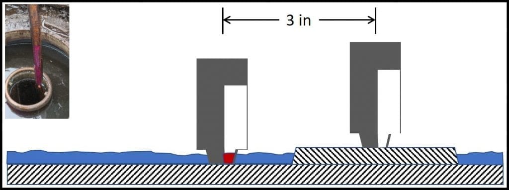
I recently received a question regarding the use of one tank-stick to measure multiple tanks. The question was: “if you stick a tank that is contaminated into the next tank, will it contaminate the second tank?”  That is: can the microbial load carried over from UST to another, on a gauging stick, infect the second UST?

Given how much press there has been lately about how easy it is to spread disease through brief, hand contact with contaminated surfaces, this is an excellent question. I thought that others who read this blog might be interested in the issue.

Here’s my response to the question:

Interesting question!.

No doubt your are extrapolating from your general understanding of how diseases can be easily transmitted either by the traces we transfer from first contacting a contaminated surface and then eating a sandwich – thereby ingesting the microbes we just transferred from our hands to the sandwich. Or, perhaps a better example is how easily viral diseases are transferred by mosquitos. A fraction of a mL of mosquito saliva can transfer a sufficient number of viruses from an infected host to a new victim.

Anything is possible, but there are a number of factors that reduce the likelihood of a gauging stick being the primary vector for microbial contamination transmission among fuel tanks:

• If a technician is using water paste, they are likely to wipe down the stick between tanks.
• Fuel is volatile; evaporation after the stick is pulled from a tank is likely to desiccate (dry out) any microbes that adhered to the stick while it was in the tank. If they are not already in a dormant state, the microbes adhering to the stick won’t have had sufficient time to transform from the active (vegetative) to dormant state before the product evaporates. Even though diesel evaporates more slowly than gasoline, it acts as a desiccant (that’s why vegetative microbes are not found in fuel that doesn’t have dispersed water present).
• Fuel systems are more hostile environments than human bodies. In microbiology we have a concept of minimum infectious dose. Typically that minimum is in the thousands or millions of cells. If the number of cells transferred is below the minimum infectious dose, then the population will most likely die off rather than seed the development of a new population in an uninfected tank that is gauged after an infected tank has been gauged.

Also, consider volumes.
• Water: 100 ppm water in 10,000 gal fuel = 1 gal water. If only 10% of that dissolve/dispersed water settles out, that’s 0.1 gal/delivery. A tank receiving only 1 delivery/wk will accumulate >5 gal/year in free-water. My 10% dropout rate is based on daily deliveries, so it’s more likely (and common) to see closer to 300 gal/y.
• Air: this might be changing as newer vapor recovery and vent systems replace current systems, but the volume of air entering a tank equals the volume of fuel withdrawn. These systems do not scrub water, pollen or dust from the air. A USAF global fuel system survey completed about 10 years ago determined that the profile of microbes found in fuel tanks closely mimicked that found in the nearby air (the research team took air samples and tank bottom samples). The research team reported much closer relationships between what they found in the air near fuel tanks and what they found I fuel tanks, than between the fuel grade and microbial community profile. These results – of course – strongly supported the hypothesis that tank vents are a (if not the) major source of microbial contamination in fuel tanks.

The next time I’m in the field performing a microbial audit of fleet or retail sites, I’ll test sounding sticks before and after using them to measure bottoms-water and product. If I find that sounding sticks are indeed picking up significant microbial loads, I’ll report that at a D02.14 Fuel Microbiology meeting, and might even write a paper on the issue.

FUEL & FUEL SYSTEM MICROBIOLOGY PART 11 –TEST METHODS – BOTTOM SAMPLE CHEMICAL TESTS

We are progressing from test methods that do not require any equipment (other the tools you need for sample collection) to those that require increasingly expensive tools. You can complete basic gross observations by relying on your eyes and nose. The physical tests I suggested in Part 10 require simple tools; including a magnetic stirring bar retriever, disposable syringes, filter pads and in-line filter holders. In this blog, I’ll discuss a couple of simple chemical tests. However, with one exception, the devices used to run these tests cost a few hundred dollars. This means that under most circumstances, I’ll be writing about tools that condition monitoring service teams, rather than individual site owners, should have on hand.

Water paste is the exception I was referring to above. I hope that if you are reading this blog, you are familiar with water paste and how to use it to detect bottoms-water. For readers who are unfamiliar with it, water paste is a thick substance that can be applied to the bottom of a sounding stick or gauge bob (fig 1). Note that if the gauging stick does not contact the tank’s actual bottom, water that’s present might go undetected.

Fig 1. Using water paste to detect bottoms-water. Left inset: gauging stick with bottom 6 inches coated with paste. The paste had been white, but had turned purple after having been lowered to the tank bottom and removed. The purple color change indicated that there were at least 6 inches of bottoms-water in the tank. Many UST have strike-plates under the fill-line. In this schematic, the UST has 0.25 inches of water. Because the strike-plate is 0.5 inches thick, gauging fails to detect the water. Had the stick contacted the UST bottom, just beyond the strike plate, the paste would have shown that 0.25 inches of water were present.

Why do I list water-paste use as a chemical test? Because the color change is a chemical reaction.  Also, if there isn’t any bottoms-water in your bottom sample, you cannot run either of the other two tests I’m covering in this post.

Point of nostalgic disclosure: the chemical tests that I am about to describe used to be more useful than they are now. Many fuel additives can move from fuel into water. This process is called partitioning. Let’s say that a particular additive is 100% soluble in fuel and 20% soluble in water. Whenever a fuel tank has any free-water, the additive will partition into the water until its concentration in the water is 20%. Keep in mind that in a UST with 7,000 gal of fuel and 70 gal of water (yes, that’s a lot of water!) the fuel to water ratio is 700 to 1. This means that even though the additive’s concentration is 20% in the bottoms-water, only an immeasurably small amount of the additive has partitioned out of the fuel. The fuel’s chemistry isn’t affected, but the water’s chemistry is. Let’s see how this affects pH and total dissolved solids (TDS).

pH measurement provides an indication of an aqueous solution’s acidity.  pH ranges from 0 to 14; with pH = 7 being neutral, pH <7 being acidic, and pH >7 being alkaline. The lower a solution’s pH, the more acidic it is. For example, the pH of stomach acid is in the 1.5 to 3.5 range (it’s essentially hydrochloric acid). Conversely, the higher the pH of a fluid, the more alkaline it i(bleach’s pH = 12). Historically, bottoms-water pH <6 was a good indicator of microbiological activity (microbes produce a variety of acids).  Although pH <6 still suggests microbiological activity, some fuel additives act as buffers – they prevent pH change.  Fig 2 illustrates the difference between adding acid to unbuffered water and adding it to buffered water.  The pH eventually falls in both cases, but when buffer is present, it takes substantially more acid to get to the same pH.  This means that in today’s fuel systems, pH drop is a later problem indicator than it was in the days before there were as many additives that partitioned into the water.

Fig 2. Buffer effect. Acid is added to two aqueous fluids; both with pH = 6.8. Fluid a is unbuffered. There is a straight-line relationship between the volume of acid added to the sample and its pH. Fluid b is buffered. Its pH does not begin to change appreciably until after 12 mL of acid have been added.

The easiest way to measure bottoms-water pH is to use pH paper (available from scientific supply distributors). Transfer a few mL of bottoms-water into a clean test tube or other small container. Dip a pH test strip into the water. After a few seconds, compare the color on the test strip against the color comparison chart provided with the test strips (fig 3). Generally, it’s sufficient to use tests trips that give whole pH unit results (fig 3a). If you want more precision, you can run a second test using pH paper that detects 0.2 pH differences (fig 3b). Digital pH meters (fig 3c) are generally more precise (reading to 0.01 pH units) than indicator strips. However, meters are more expensive than disposable test strips. Additionally, if meters are not kept clean and calibrated, they can give you precise, but inaccurate results.

Fig 3. pH test kits: a) broad range (pH 0 to 13), pH test strips with 1 pH unit precision; b) narrow range pH test strips with 0.2 pH unit precision; c) hand-held pH meter.

The final chemical test I’ll discuss today is TDS. As the name implies, TDS include all dissolved chemicals (organic and inorganic) in bottoms-water. Before the late 1990’s, typical gasoline bottoms-water TDS were in the 150 mg L-1 to 250 mg L-1 range and diesel fuel bottoms-water TDS were in the 250 mg L-1 to 500 mg L-1 range. High TDS concentrations would signal the presence of dissolved metals (corrosion byproducts), microbes and their metabolites, or both. However, the increased use of fuel additives that can partition into the water has translated into TDS >2g L-1 in both gasoline and diesel fuel bottoms-water. This high background TDS concentration can mask the contribution of microbes and corrosion to the total. There is a work-around, but the details are beyond the scope of this blog post.

TDS can be measured by weighing the residue that’s left behind after the fluid has evaporated away. However, TDS is directly related to conductivity (the ability of a material to carry an electrical current). The easiest way to measure TDS is to use a handheld meter (fig 4). Most meters offer the option of showing either conductivity (µS cm-1) or TDS (mg L-1).

Fig 4. Conductivity meter.

If you collected a good sample, by the time you have collected water level, pH, and TDS data, you know quite a bit about the condition of the fluids in your tank. You are at the “if it walks like a duck and quacks like a duck…” point of your field testing effort. You should be 90% certain of whether you have uncontrolled microbiological contamination (MC) in your system. Final confirmation depends on microbiological test results. I’ll begin to discuss these in my next post. Of course, if you want to learn more now, please send me an email at fredp@biodeterioration-control.com.

FUEL & FUEL SYSTEM MICROBIOLOGY PART 10 –TEST METHODS – BOTTOM SAMPLE PHYSICAL TESTS

Let’s get physical. In Part 9, I discussed some very easy gross observation tests you can use to determine the likelihood of substantial microbiological contamination (MC) in fuel tanks (nearly everything in this blog series applies to tanks of all sizes from power tool tanks (<1 gal) to refinery bulk storage tanks ( as large as 500,000 bbl).This post introduces a couple of very simple physical tests you can run on bottom samples to detect fuel system damage that might be related to uncontrolled MC (biodeterioration).

First, I’ll repeat something I’ve written previously: many individual biodeterioration symptoms are identical to the effects of non-biological processes. Do not draw conclusions from the results of any individual test. Treat each result as a piece of puzzle. At the same time, don’t forget: if it walks like a duck and quacks like a duck… What makes identifying MC and biodeterioration different, is that most of us can recognize a duck when we see one. Few of us have been taught how to recognize biodeterioration when we see it.

The first physical test I’ll review in today’s blog is rust. If you have no particles visible in your bottom-sample, there’s no need to run the test. However, if you see particles, a sludge/sediment layer, or if the sample contains opaque bottoms-water, this is a quick test to determine whether the sample contains rust particles. The one tool you need for this test is a magnet. I use a stirring bar retriever – a 12 in long, Teflon (Teflon is a registered trademark of Chemours’ polytetrafluoroethylene – PTFE) rod, that has a magnet at one end. You can also use an uncoated magnetic retriever or screwdriver with a magnetized head (both available at most hardware stores). You simply dip the magnet into the sample, gently swirl it around the sample bottle’s bottom, pull the magnet out of the bottle, and look at it. Compare what you see with the five examples shown in Fig 1. If the amount of rust is similar to that shown in photos 1 and 2, you probably do not have a corrosion problem. If you have lots of magnetic particles on the magnet (photos 4 and 5), then you most likely have a corrosion problem. Photo 3 suggests that there some corrosion, but it is not yet serious. Note: These photos are from bottom samples I took from a fiber reinforced polymer (FRP) tanks. Don’t forget that even FRP tank fuel systems have metal components that can rust.

Fig 1. Bottom sample, magnetic particulate load. 1 & 2: negligible contamination; 3: moderate contamination; 4 & 5: heavy contamination.

The second test is just a bit more technical. To run this test, you’ll need a disposable, polypropylene, 50mL syringe; a 25 mm, in-line filter holder, 25 mm glass fiber filters, and a suitable waste receptacle for capturing the filtered fluid.
    Step 1: place a glass fiber filer into the filter holder.
    Step 2: remove the plunger from the syringe and attach the filter to the end of  the syringe.
     Step 3: dispense either 25 mL of fuel or 25 mL of bottoms water.
     Step 4: Replace plunger into the barrel of the syringe and filter the fluid.
     Step 5: remove filter from the filter holder and look at it; comparing its appearance with the illustrations in Fig 2.

Just as with Fig 1, the higher the score, the more likely you have substantial MC in the system.


Fig 2. Quick & dirty fuel particulate test. 0: clean; 1 & 2 moderate contamination;
3 through 5 heavy contamination.

Two quick and simple tests: One detects magnetic particulates and the other detects all particles that are trapped on the filter. A more formal version of the filtration tests includes weighing the filter before use, drying the filter and weighing it again after the residual fuel or water has evaporated off. After subtracting the filter’s original weight from its final weight and dividing by the volume filtered (sometimes you can push all 25 mL through the filter) you get particulate concentration in mg/mL. The lower the number, the better (ASTM D975 Specification for Diesel Fuel Oils; has a specification of ≤0.05 % by volume; this is  ≤50 mg/mL).
These two physical tests build on the information you get from gross observations. If both the gross observation and physical test results indicate MC, then it’s a good idea to have a couple of chemical tests run. I’ll discuss these in my next post. If you are impatient and would like to learn more now, please send me an email at fredp@biodeterioration-control.com.


FUEL & FUEL SYSTEM MICROBIOLOGY PART 9 –TEST METHODS – BOTTOM SAMPLE GROSS OBSERVATIONS

Beginning with this post, I’m moving into Phase 3 of this series. In the first five posts, I introduced the issues that make fuel system microbiology condition monitoring important.  In Part 6 through 8 I covered the foundational concepts of sampling and testing.  Now it’s time to talk about actual test methods. The take home lesson here is that you can detect microbial contamination without having a lot of technical training or investing in expensive laboratory facilities.

Gross observations are tests that rely only on our senses.  We look at, sniff, and, perhaps, touch samples to determine whether they are likely to be heavily contaminated.   We begin by obtaining a useful sample.  If you are not sure what I mean by useful sample please read my 28 November 2016 blog post on sampling.

Bottom-sample gross observations work best if you collect the sample from the lowest point in the tank.  Underground storage tanks settle unpredictably.  The first-time a UST is filled, its 90,000lb weight compresses the backfill on which it rests.  Regardless of how well the backfill is prepared, some areas will be softer than others.  The UST will continue to compress the backfill for years.  This means that it is important to check its trim (angle at which the UST lies) annually.  To do this, stick the tank at three points: fill end, turbine end and automatic tank gauge ATG – (usually this will give your fuel levels at each end and the center).  The fuel level will be greatest at the UST’s low point.  Although most UST are installed to be low at the fill end, Murphy’s Law seems to dictate that much of the time, they settle by the turbine end.  Best design is to have an inspection port in the turbine well (figure 1). If find that the UST’s low point is at the turbine end but you can’t sample from that end routinely, sample from the ATG well.  Pulling the ATG will give you a chance to look at the ATG’s water float.  If it looks like figure 2, you most likely have a microbial contamination problem.

Figure 1. Turbine well showing 4in inspection port just left of center.

Figure 2. ATG water float covered with microbial contamination.

The two samples most likely to provide the best clues about a fuel system’s condition are bottom samples and components (filter, flow-control valve, automatic tank gauge float, etc.).  Let’s focus on bottom samples.  If you pull a sample from a tank’s lowest point, and get a sample that looks like figure 3, you can be fairly certain that you do not have a severe microbial contamination issue.  On the other hand, if your sample looks like the one in figure 4, there’s a >90% probability that the system is heavily contaminated.  Microbes produce chemicals that can emulsify fuel.  Hazy fuel or a third layer, between the water and fuel is a sure sign of microbial activity – particularly if the middle layer sticks to the side of the sample bottle as it does in figure 5.

Figure 3. UST bottom sample: there’s no water, and the fuel is clear and bright; water-white.

Figure 4. UST bottom sample; A thick rag (invert emulsion) layer separates the hazy fuel from the very turbid, bottoms-water.

Figure 5. UST bottom sample: rag layer (looks like a hanging drape)
adheres to the sample bottle wall.

Quick, simple, gross observations provide reliable indications of uncontrolled microbial contamination.  If your eyes tell you the system is clean, then you don’t need to do any more microbiology testing.  If gross observations signal microbial contamination, the next step is to confirm what your eyes are telling you.  I’ve just scratched the surface in this blog.  If you’d like to learn more, please send me an email at fredp@biodeterioration-control.com.

FUEL & FUEL SYSTEM MICROBIOLOGY PART 8 – CHOOSING TEST METHODS B

STP spill containment well.  Good news: well has a 4 inch port for testing bottoms-water height and collecting bottoms samples.  Bad News: there is lots of corrosion.

The canary in the coal mine….

In my last post, I discussed the kinds of questions that should be asked before deciding on what tests to run and how frequently to run them.  Now I’ll share my condition monitoring (CM) philosophy with you. I’ll list them as axioms – statements that should seem obvious to the most casual of observers. 

Axiom 1: For most frequent testing, rely on methods that are easy to perform and interpret.  The flow-rate example that I shared in Part 7 (16 February 2017) illustrates this point.  You can test dispenser flow-rate while filling your vehicle.  The only test equipment you need is a stop watch, or flow-rate APP (I don’t want to be commercial here, but I know of at least one fuel system service company that offers a free, dispenser flow-rate APP). 

Axiom 2: The tests you run most frequently should be your canaries in the coal mine1.  I call these simple, frequently run tests 1st Tier tests.  They don’t tell you much about why there is a problem, but signal either that a problem exists, or that the risk of a problem developing has increased.  Examples of other 1st Tier tests include:

  • Bottoms-water detection, by water-paste on fuel gauging stick or sounding bob.
  • Standing water in spill containment wells.
  • Broken spill containment well covers.
  • Heavily corroded submerged turbine pump (STP), turbine distribution manifold (see photo above).

The common feature of these tests is that they require very little technical training or test equipment.

Axiom 3 (repeat from Part 7): Every parameter that you test must have control limits! You need to know what is normal and what isn’t.  I like the green, amber, and red light approach. 

  • When conditions are normal, you have a green light.
  • When conditions are not quite normal, but operations don’t seem to be affected, you are in the amber light zone. This is the time to run additional tests or schedule preventive/early corrective maintenance. This is the zone that links CM to predictive maintenance (PdM – see Part 5).
  • The red-light zone indicates that you are having problems. You need to schedule corrective maintenance as soon as possible. When your site has a well-planned, well executed CM program, you never get red zone test results. Red-light results signal both operational and PdM program problems.

Axiom 4: 1st Tier, amber-light results should trigger either maintenance actions or 2nd Tier tests.

  • Action example: if you detect water in a spill containment well or tank bottom, remove it. There’s no need for additional testing to help you determine the best course of action.
  • 2nd Tier testing example: If your dispenser flow-rate <80% of maximum, use 2nd Tier testing to determine why.  Remember: slow-flow is not the same as a plugged filter!  There are several chokepoints (for example: screens) between the STP and dispenser nozzle.  Moreover, slow-flow after a 500 000 gal of fuel have passed through a dispenser filter tells a much different story than slow-flow after 50 000 gal have been filtered (see the flow-rate testing example in Part 7).

Axiom 5: 2nd Tier tests should be diagnostic, but sufficiently easy to perform so that a trained technician can complete the testing on-site. In most cases, 2nd Tier test results provide sufficient information to guide maintenance actions.  I break 2nd Tier tests into four categories, and will discuss each category in more detail in the next four MICROBIAL DAMAGE blog posts. I list the categories here:

  • Gross observations
  • Physical tests
  • Chemical tests
  • Microbiological tests

There are rare occasions when the 2nd Tier test results are inconclusive.  Additional testing is needed to diagnose what’s going on.  In most cases, 3rd Tier tests are run at specialty testing labs.  These are labs that have particular expertise in fuel, corrosion, or microbiological testing.  Examples of 3rd Tier testing include:

  • Corrosion deposit analysis
  • Fuel property testing (this typically includes tests listed in ASTM fuel specifications)
  • Bottoms-water chemistry testing
  • Fuel or bottoms-water microbiology testing (detailed tests to determine the types of microbes present)

One very rare occasions, 4th Tier or 5th Tier tests are run to gain a deeper understanding of the processes that increase operational risks.  These higher tier tests are typically run as part of research efforts rather than in direct support of troubleshooting.  There is still quite a bit that we do not know about what causes fuel quality problems and fuel system failures.

As I have noted in previous posts in this series, in each post, I’m peeling back another layer of a complex onion.  If you are impatient and want to learn more now, don’t hesitate to contact me at fredp@biodeterioraiton-control.com. 

1 In the days before electronic oxygen and explosive gas detectors, miners would use canaries as hazard alarms.  If methane or carbon dioxide concentrations became too high, the canaries would die.  The canaries’ sudden silence would alert miners that they needed to evacuate the mine – high methane meant high explosion risk! (more…)

FUEL & FUEL SYSTEM MICROBIOLOGY PART 7 – CHOOSING TEST METHODS A

TEST METHOD SELECTION

How do we select condition monitoring tests?

Parts 3 and 4 of this series introduced the issue of test method selection. Starting with Part 7, I’ll spend the next few posts drilling down into different testing options when you want to evaluate fuel system microbiological contamination.
Today let’s start with two questions. These are the two questions that should drive most predictive maintenance test decisions:
What do I need to know to be sure I have a microbial contamination problem?
→What will I do with test results?
Although microbiology data are useful – even important – they are only part of the story. This means that the first question’s answer is not necessarily microbiology data. In this blog post, I’ll focus on the first question.

What do I need to know to be sure I have a microbial contamination problem?
There’s an old joke in which one person asks another: “Why do you always answer my questions with a question?”. The person to whom the question was posed responds: “Do I?” In the same vein, the answer to What do I need to know? is What will you do with the results? There is no benefit to running any test if the results do not drive some action when the results indicate that conditions are not normal (i.e.: in specification). This means that when a technician is tasked with running a test, they need to know three things:
       • How to run the test
       • What the test results indicate
       • The next action to be taken if the results indicate that conditions are not normal.
Running tests – every test method should be detailed in a standard operating procedure (SOP) document. This SOP can be an ASTM, PEI or other method developed as a consensus standard. It can be a method developed by an employer. As I noted in Part 5, the Navy uses Maintenance Requirement Cards (MRC). A well written SOP lists all materials, supplies and tools needed to perform the task. It lists both hazards and potential interferences. It then provides detailed instructions for how to complete the task. Next, test method SOP specify what to report and how to report the results plus supporting information. Finally, the test method SOP provides guidance on how to interpret the results and what action to take.
What the results indicate – some methods generate numerical data. For example, one of the easiest tests to run is dispenser flow-rate. The technician either determines how long it takes to dispense a specified volume of fuel, or determines how much fuel is dispensed during a fixed time. The results are reported as gallons (or liters) per minute (gpm). Without some context, the results are not particularly helpful. However, we can assign attribute scores to flow-rate ranges; for example:
       • 8 gpm ((30 l/min) to 10 gpm (38 l/min): normal;
       • 6 (23 l/min) gpm to <8 gpm: moderately reduced; and
       •<6 gpm: severely reduced.  For fleet operations, the breakpoints might be 36 gpm (136 l/min) and 24 gpm (91 l/min). 

Having assigned attribute scores to our raw data, we know that the flow-rate of a retail dispenser dispensing fuel at 4 gpm (15 l/min) is severely reduced. Some action is needed.

What action is needed? – most often – particularly for quick and dirty tests – the action triggered by a test result that indicates that there is a problem, is additional testing. In our dispenser flow-rate example, the severely reduced flow can be a symptom of different causes; including microbiological contamination.

For example, if the test is run when several dispensers are being operated, the pump might not have sufficient power to deliver full flow to all active dispensers. An under-capacity pump has nothing to do with microbiological contamination. Alternatively, reduced flow could be a symptom of contamination. Again, not all contamination is microbial. Moreover, the assumption that slow-flow is due to filter plugging can be wrong. This leads to a set of IF/THEN instructions:

     • IF flow <6 gpm, THEN retest after confirming that no other dispensers are operating.
     • IF flow <6 gpm when no other dispensers are operating, THEN replace filter and retest flow rate.
     • IF flow is <8 gpm after replacing filter; THEN clean dispenser prefilter (screen) and retest flow rate.
     • IF flow rate is <8 gpm after cleaning prefilter; THEN test leak detector, replace if necessary, and retest flow rate.
     • IF flow rate <8 gpm after testing/replacing leak detector; THEN test/repair/replace submerged turbine pump and retest flow rate.

Notice that in each case, the level of effort is greater and the flow rate is retested after the action has been completed.
By now, perhaps you are wondering: All this is interesting but what do I really need to know to be sure I have a microbial contamination problem? Stay tuned. In Part 8, I’ll offer some approaches to how you can answer that question.

Flow-rate testing as I’ve described here is one example of tiered testing. Here I reran the same test after taking increasingly complex maintenance actions. In future posts, I’ll write about more tiered testing in which the results from a simple test trigger the need to run a more complex test. I’ll also discuss individual test methods and share my opinions about their respective advantages and limitations. If you are impatient and want to learn more now, contact me at fredp@biodeterioraiton-control.com.

VENDOR VIEW: FUEL SYSTEM BUGS DRAIN REVENUES

Twenty years ago I had a series of retail fuel system articles published in National Petroleum News. Ten years ago, I wrote a Looking Back preface for each of the original articles, and sent the updates to a selected distribution list. Quite a bit has changed since I wrote the original series and the 10-year updates. I’ve just launched a new series for publication in Fuel Marketing Reporter. This series will follow a series of themes similar to those I’m addressing in my Why is Microbial Damage to Fuel Systems so Hard to Detect blog series. You can find my new article: Vendor View: Fuel System Bugs Drain Revenues at Fuel Market News.

FUEL & FUEL SYSTEM MICROBIOLOGY PART 5 – PREDICTIVE MAINTENANCE (PdM)

I introduced predictive maintenance (PdM) in my last post. Because I didn’t mention preventive maintenance (PM) in that post, I used “PM” as an abbreviation for PdM. After reading Part 4, one of my readers asked me to explain the difference between PM and PdM. I’ll oblige that reader in this post.
The very first collateral duty I was assigned when I reported aboard my first ship, as a fresh-caught Ensign, in January 1971, was to implement the Navy’s new Material Maintenance Management (3-M) System which had arrived onboard days before. The Preventative Maintenance System (PMS) was a major sub-system of 3-M. There it sat in nearly a pallet load of corrugated cardboard boxes; all but one of which was filled with Maintenance Requirement Cards(MRC).
Each MRC provided the details needed to enable a sailor (sometimes more than one sailor) to complete a specific preventive maintenance item. It listed: safety considerations, all materials needed (tools, parts, etc.), estimated time to complete, a step-by-step protocol the qualifications (pay-grade(s)) the sailor(s) needed to have before attempting the maintenance action. The remaining box contained the preventive maintenance scheduling guidance. Each maintenance activity covered by an MRC, was assigned a frequency: daily, weekly, monthly, quarterly, annually, or as required. The Chief Petty Officers and Leading Petty Officers of each division (team of sailors with specific rates – job titles and skill sets) were to develop and maintain weekly, monthly and quarterly charts showing scheduled and completed maintenance. For some reason, I decided to calculate the total number of person hours needed to compete all of the PM requirement. I then computed the total number of person hours available, based on the number of sailors serving on the ship. It turned out that the folks who had developed the 3-M PMS had not done a similar calculation. Had all hands spent 24h/d x 7 d/w x 52 w/y they would have provided just about enough person-hours to complete 40% of the PM labor. Such was my introduction to PM.
Don’t get me wrong, PM was a great innovation for its time. The predetermined maintenance item frequency was based on someone’s best estimate of what needed to be done to minimize the risk of equipment failure. However, it was not data driven. In fact, the 3-M system had a fairly effective feedback component, and before many years passed, the Navy learned that in some cases, maintenance actions actually increased failure risks. I suspect that early PM adapted in industry learned some of the same lessons. Eventually, PdM succeeded PM. In contrast to PM, in which maintenance actions are all given the same priority and are timetable driven, PdM uses trend analysis, condition monitoring (CM) data, asset assessment and cost impact analysis to determent when preventive maintenance actions are needed. The end objective is the same for both PM and PdM, but the latter makes much better use of available resources.
So how do we design fuel system predictive maintenance programs that provide a high return on investment?
Let’s start with cost impact analysis. My experience with microbial audits at fuel retail sites suggests that annual corrective maintenance costs at heavily contaminated sites run $1,500 to $2,500 more than at sites with negligible microbial contamination. I’ve also found that at sites where cars line up to fill-up, 8 gpm dispenser flow rates (instead of 10 gpm) translates into 62,000 fewer gallons sold per dispenser per year. Today, gasoline and diesel are both selling for $2.45/gal. At that price the fuel not sold is worth $152,000. That is opportunity cost. Multiply that number by the number of dispensers on site and the opportunity cost becomes substantial. If the site also has a C-store, estimate the impact of reduced dispenser flow rates on customer satisfaction and C-store traffic/purchases. All you really need to know at the outset is your typical dispenser flow rate, your current fuel price and the number of hours per day during which drivers have to wait in line before pulling up to a dispenser.
In my next What’ New post, I’ll discuss some basic CM tools. In the meantime, if you’d like to learn more, reach out to me at fredp@biodeterioration-control.com.

FUEL & FUEL SYSTEM MICROBIOLOGY PART 4 – MORE ON TESTING

drunk-looking-for-keys

Are we like the drunk who looks for his keys under the lamppost (if you don’t now this shaggy dog story, he had dropped them in the nearby dark ally, but chose to look where there was more light…)?

In my last What’s New post I quoted Daniel Kahneman: “What you see is all there is (WYSIATI).”  In this post I’ll explore the concept a bit further.  First, I will review some of the essential concepts I’ve covered in my three most recent, previous posts.  Apropos of EPA’s observation that at 83% of the fuel retail sites with moderate to severe corrosion, the owners were unaware of the problem.  That’s like saying that 83% of people with moderate to severe heart disease are unaware of their condition (there is a reason that heart disease is called the silent killer).  These folks simply walk around like heart attack time bombs; confident that they are not at risk – until the moment they collapse and must be rushed to the hospital.  In the case of heart disease, there is a considerable amount of public outreach to help educate people about the importance of routine health examinations.  These examinations are performed to detect incipient disease and to identify actions that can be taken in order to reduce the risk of the disease causing major health issues. 

Effective condition monitoring programs serve the same purpose.  In the manufacturing world, asset-value based predictive maintenance (PM) is the currently accepted best practice.  PM is based on the proven return on investment from timely and effective condition monitoring that drives equally timely and effective maintenance actions in order to maximize equipment performance and performance life.  Unfortunately, this approach is not broadly embraced within the petroleum retail community.  What we generally accept as condition monitoring focuses on detecting damage after it has occurred: WYSIATI – until we see damage, we assume that it can’t exist.  In my Microbial Damage – Part 2, What’s New post I discussed the effect of collecting the wrong type of sample.  In may last post, I compared the ability of different types of microbiological tests to detect microbial contamination when it was present in the sample. 

In the fuel retail sector, we have a tendency to wait until we have had a failure (perhaps as minor as a broken well-cover, or as major as a leaking UST), a tendency to collect the most convenient sample rather than the one most likely to harbor microbes (like looking for our keys under the lamppost, where there is light, instead of in the dark ally, where we dropped them), and we tend to use a microbiological test method (culture testing) that has been around for nearly a century (remember, culture testing is unlikely to detect more than 0.1% of the microbes present in any fuel-system sample).  We then feel confident that our fuel systems are risk-free.  Here is today’s take home lesson: negative (below detection limit) microbiological test results provide much less information about contamination than do positive results. 

So how do we design fuel system predictive maintenance programs that provide a high return on investment?  I’ll offer some thought about this in my next What’s New post.  In the meantime, if you’d like to learn more, reach out to me at fredp@biodeterioration-control.com.

FUEL & FUEL SYSTEM MICROBIOLOGY PART 3 – TESTING

.

How much of the total microbial load each type of test detects.


I’m starting this post with an illustration from one of my recent presentations (click on the image to enlarge it). The quote is from Daniel Kahneman’s book: Thinking, Fast and Slow. It reminds us of how often our perceptions are much more limited than we realize. Let’s turn to the circles to the right of the quote.

(more…)

OUR SERVICES

  • Consulting Services
  • Condition Monitoring
  • Microbial Audits
  • Training and Education
  • Biocide Market Opportunity Analysis
  • Antimicrobial Pesticide Selection

REQUEST INFORMATION


    captcha