Archive for the ‘Fuel Microbiology’ Category


FUEL & FUEL SYSTEM MICROBIOLOGY PART 18 – PREVENTING MICROBIAL DAMAGE TO FUEL SYSTEMS PART 1

Disclaimer:

I’ll open this post with a disclaimer. Microbes are ubiquitous. There are extraordinarily few habitats on earth where thriving, microbial communities have not been detected. In practical terms, this means that it is unlikely that operators will ever have a completely sterile fuel system or that they will reduce their fuel system biodeterioration risk to zero. Biodeterioration can still occur in the best maintained fuel systems. However, the risk of it occurring in an inadequately maintained system is much more likely.

Biodeterioration:

I’ll also take this opportunity to remind readers that biodeterioration (damage caused by organisms) and bioremediation (using microbes or other organisms to degrade or remove toxic or noxious chemicals) are the flip-sides of the biodegradation coin (figure 1).

Figure 1. Just as the two sides of a coin are its obverse (front) and reverse (back) sides, the two sides of biodegradation are bioremediation and biodeterioration.

Microbes degrade fuel quality and fuel system components. In high-turnover retail systems, product deterioration is unlikely. I consider any tank that is refilled at least weekly to be a high-turnover (or high-throughput) system. The time that product spends in the storage tank is too short for degradation to occur. Studies that investigate the rate at which microbes change fuel chemistry, typically show substantial changes after a month or longer. Consequently, fuel in tanks used for emergency generators, or seasonally operated equipment is at greater biodeterioration risk than fuel in retail underground storage tanks (UST), or frequently operated vehicles. That’s all I want to say about fuel biodeterioration for now. I’ll return to the topic in a future blog post.

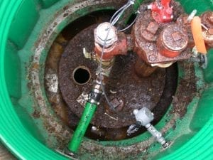
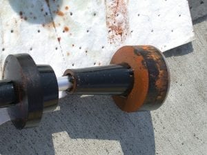
For now, I’ll focus on fuel system biodeterioration. Most of the damage caused to fuel system components is caused by biofilm communities (see post #16 https://biodeterioration-control.com/2017/11/). Microbes cause damage either directly or indirectly (more on this in a future post). The most obvious indications of biodeterioration are filter plugging and corrosion. Although it’s typically the first indication of a biodeterioration problem, filter plugging is a late symptom. I often compare it to a heart attack; a late – but often first recognized – symptom of coronary disease.

So how do we substantially reduce fuel system biodeterioration risk? Step one is cost-effective condition monitoring (CM). Step two is cost-effective predictive maintenance (PdM; see https://biodeterioration-control.com/microbial-damage-fuel-systems-hard-detect-part-5-predictive-maintenance-pdm/). The former drives the latter. Why do I emphasize cost-effectiveness? As I see it, there is as little justification for investing $10,000 per year to detect problems that might cause $1,000 per year of damage, as there is in refraining from spending $10,000 per year to detect problems that could cost $100,000 per year. I’m not suggesting that any fuel system CM program should cost $10,000 per year. An effective program can cost less than $2,000 per year. My point here is that before setting up a CM/PdM program, stakeholders should invest a bit of time and effort to determine their actual annual biodeterioration-related costs.

Opportunity Cost:

Nearly two decades ago, I first argued that a 10% flow-rate loss at high-traffic, retail sites, can easily translate to more than $100,000 per dispenser per year opportunity cost (Passman, F.J., 1999. “Microbes and Fuel Retailing: The Hidden Costs of Quality.” Nat. Petrol. News 91 [7]: pp: 20-23). My model did not include lost C-store revenues related to customer discontent with their fueling experience. Retailers who have tested my model have invariably been shocked by the huge impact of seemingly minor flow-rate reductions on fuel sales volumes. I’m still trying to understand the psychology behind retailers’ general reluctance to even test my model (for model details, contact me at fredp@biodeterioration-control.com). Bottom line: the return on investment (ROI) for well-designed and executed, CM can easily be >$1,000 return on each $1 invested.

Condition Monitoring:

In Parts 2 through 18 of this series, I’ve written about the details of condition monitoring. I won’t repeat that information here. Instead, I’ll offer a few basic guidelines:

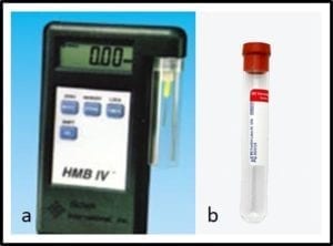
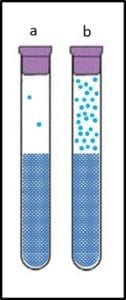
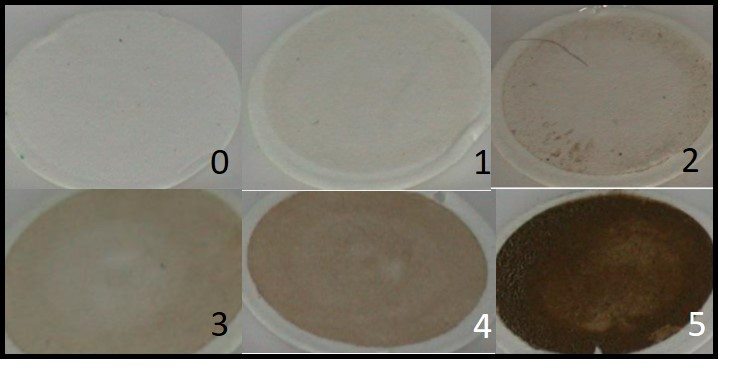
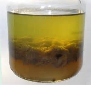
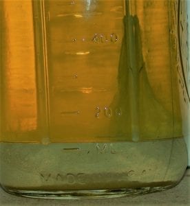
1. Testing hierarchy – CM plans should include two or more tiers. Tests that are easiest and least expensive to perform should be done most frequently (checking UST for bottoms-water accumulation and dispenser flow-rate checks are great examples of Tier 1 tests). Tier 2 tests include bottom-sample visual inspection (optimally, samples should be collected from the fill, automatic tank gauge, and submerged turbine ports). A simple microbiological test (for example ASTM D7687) is indicated whenever the bottom-sample is turbid or when it includes water. When Tier 2 tests indicate that the biodeterioration risk is moderate to high, Tier 3 tests (generally performed by a qualified laboratory) are used to confirm the risk.

2. Test method selection – notwithstanding the examples I mentioned under Testing hierarchy each site owner should develop a CM plan that best meets their needs. You can read my test specific blog posts (or ASTM D6469) for discussions of the benefits and limitations of each test method.

3. Testing frequency – my rule of thumb, after you have determined how often a test parameter is likely to indicate an increased biodeterioration risk, divide that period in three. That gives you the optimal test interval. Testing more often typically translates into greater costs without any real ROI. Testing less frequently increases the risk of having to perform corrective – rather than preventive – maintenance actions.

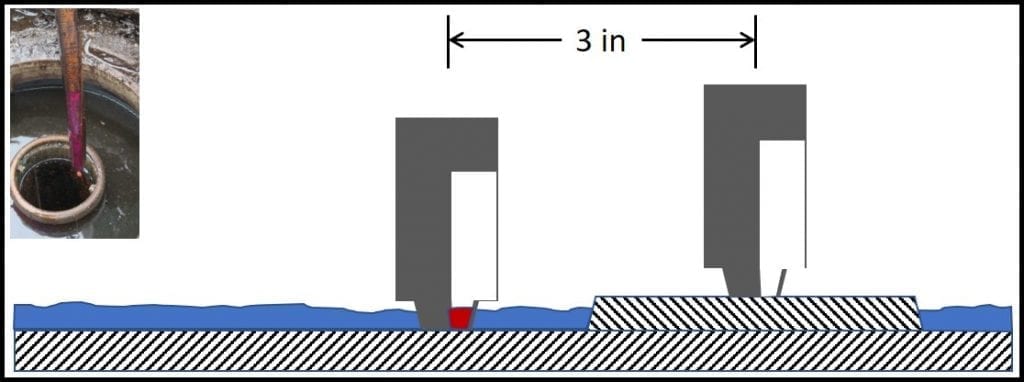
4. Understanding trends – each of the three previous guidelines depends on a basic understanding of trends. For example, even fuel with an ISO 4406 cleanliness rating of 18/16/13 (see https://www.iso.org/standard/72618.html), will eventually plug dispenser filters. Consequently, dispenser flow-rates will invariably decrease. How many operators know what normal looks like? How many have a control limit? Typically, dispenser filters can process >250,000 gal of fuel before the flow rate will fall below 7 gpm. Replacing fuel filters when the flow-rate is <7 gpm strikes a balance between the opportunity maintenance costs. Knowing whether the flow rate has fallen to <7 gpm after 50,000 gal or 500,000 gal of fuel have been filtered serves to trigger additional sampling and testing. If the amount of fuel filtered before substantial flow reduction occurs is much less than expected, then additional testing is indicated.

Summary:

In summary, microbial contamination control depends on a good CM program that is linked to a good PdM program. A reasonable investment in CM and PdM should be a fraction of the likely cost impact of not having those programs in place. A cost-effective CM program is driven by an understanding of system trends, definition of the methods that will provide the most useful, actionable information; selection of which tests to run; and determination of sampling and testing frequency. In my next blog, I’ll focus on preventive measures. In the meantime, if you have questions or comments about today’s post, please contact me at fredp@biodeterioration-control.com.


FUEL & FUEL SYSTEM MICROBIOLOGY PART 17 –TEST METHODS – GENETIC TESTING

In today’s blog, I’ll cover the lastest family of microbiology methods used for testing fuels & fuel associated water. These methods fall under the category genomics – the study of genes. Warning: genetic testing is more technically complex than the methods I’ve described in recent posts. I’ll do my best to keep the language as simple as possible.

Genetic methods have evolved substantially over the past 30 years. They all depend on the polymerase chain reaction (PCR); first reported in 1983. The common steps of all PCR methods include:

   1) Genetic material (deoxyribonucleic acid – DNA) extraction (fig 1).
   2) Heating to separation of the two strands of DNA’s double helix (fig 2) into two single-strands.
   3) Cooling and using an enzyme – polymerase – to convert each single strand back into double stranded DNA (fig 3).
   4) Repeating steps 2 and 3 until there are millions of copies of each of the DNA originally extracted in step 1.
   5) Using analytical tools to: identify the different types of DNA that were extracted from the original sample in step 1.

Fig 1. Bacterial cell lysing and ejecting its cytoplasm

Fig 2. a) DNA molecule ; b) section of DNA being denatured to two single strands.

Fig 3. Denatured DNA (left) coupled with primer and reacted with DNA polymerase to form two new double helices.

When PCR methods were first developed in the mid-1980s, DNA was extracted from colonies that had developed on nutrient agar plates (see Part 12 and fig 4). Early PCR testing revolutionized microbial taxonomy. Microbes that seemed to be closely related because of their appearance and nutrient preferences turned out to be quite distant genetic relatives. Conversely, some microbes that had historically been classified as being members of different groups, were discovered to be nearly identical genetically. However, PCR could only be used to identify microbes that formed colonies.

Fig 4. Bacterial colonies on nutrient agar.

In the 1990s quantitative-PCR (qPCR) methods were developed. In qPCR, messenger-RNA (mRNA) is extracted and used to synthesize complimentary-DNA (cDNA). The PCR process then continues as described in steps 2 through 5. The RNA used for qPCR is typically tagged with a fluorescent dye. A fluorometer is used to measure the DNA concentration as a function of time during repeated cycles of heating and annealing (steps 2 and 3). As shown in fig 5, the time required for the fluorescence to reach a threshold value, can be used to compute the amount of mRNA that was originally extracted from the sample. This, in turn provides an accurate estimate of the population density (i.e., cells/mL) in the sample.

Fig 5. DNA amplification curves: delta Rn is the amount of fluorescence detected and ct is the threshold delta Rn used to compute the DNA concentration in the original sample. The five curves show that the number of PCR cycles needed to reach ct increases as the original DNA concentration decreases.

Four molecules (nucleotides) make up the genetic code (adenosine – A, cytosine – C, guanine – G, and thiamine – T). Each three-nucleotide sequence is the code for a specific amino acid. Thus, long strings of three-letter messages specify the amino acid sequence of enzymes – the cell’s machinery for carrying out all of life’s processes. The total genome of each type of cell (operational taxonomic unit – OTU) is unique. Because each of the four nucleotides – A, C, G, and T – has a unique electrical charge, each OTU’s DNA has a unique net electrical charge. Using a technique called gel electrophoresis, after amplification (step 5) analysts can separate and isolate each type of DNA that was recovered from the original sample (fig 6). They can then sequence the genes and attempt to match the sample’s DNA against a DNA library. The result is a taxonomic profile of the microbes that were present in the original sample.

Fig 6. DNA profiling using gel electrophoresis: a) schematic illustration of process ; b) photograph of gel.

In earlier posts, I’ve referred to Donald Rumsfeld’s “unknown unknowns.” Although qPCR and, the more recently variation called next generation sequencing – NGS, is a powerful tool for studying microbial communities in fuel systems, it is probably not the last word in microbiology testing. True, qPCR detects many types of microbes that are undetectable by historically used culture methods. However, extracting DNA or RNA from cells is as much art as science. Genetic material that isn’t extracted isn’t detected. Additionally, qPCR testing depends on the use of primers – short sections of mRNA selected to either be universal (i.e., include a section of A, C, G, T basis that are believed to be present in all bacteria) or specific (i.e., include a section of genetic coding that is unique to a microbe of specific interest). Consequently, researchers are on a steep learning curve about how to select primers. As task force within ASTM D02.14 has just restarted work on a qPCR standard test method for fuels and fuel associated water. The last attempt stalled when participants could not agree on a consensus DNA extraction protocol. As the new task force makes progress I provide readers with updates. The goal is to develop a method that non-technical folks will be able to use.

In the meantime, please contact me at fredp@biodeterioration-control.com you’d like to learn more about fuel system microbiology or microbiological contamination control.

Footnotes:

Source: http://www.newswise.com/images/uploads/2013/01/9/lysis_cover.jpg.
Source: http://www-nmr.cabm.rutgers.edu/photogallery/proteins/gif/dna.gif.
Source: https://laboratoryinfo.com/wp-content/uploads/2015/07/Polymerase_chain_reaction.svg_.png.
Source: https://www.microbiologyinpictures.com/bacteria-photos/escherichia-coli-photos/e.-coli-staphylococcu-aureus-colonie.jpg.
Source: https://media.nature.com/full/nature-assets/leu/journal/v17/n6/images/2402922f5.jpg.
Source: http://science.halleyhosting.com/sci/ibbio/biotech/pics/electrophoresisnotes.gif.
Source: https://78.media.tumblr.com/tumblr_lwthmyKO441qzcf71o1_500.gif.

FUEL & FUEL SYSTEM MICROBIOLOGY PART 15 – TEST METHODS – HOW DO WE DETECT BUGS ON SURFACES?

In my August post (https://biodeterioration-control.com/microbial-damage-fuel-systems-hard-detect-part-14-test-methods-still-microbiological-tests/), I discussed using ASTM D7687 to quantify microbial loads (AKA bioburdens) in liquid samples – fuels and fuel associated water. This post will focus on surface samples.

Generally speaking, microbes tend to be most abundant on surfaces. By some estimates, in any given system, for every microbe floating in the bulk fluid, there are 1,000 to 1,000,000 growing on surfaces. These surface microbes are invariably part of biofilm communities. I’ll discuss biofilms in more detail in a future post. For now, it is sufficient to understand that biofilms are slime-encased microbial communities growing on surfaces (fig 1). It is much easier to grab a fluid sample than a surface sample. Consequently, most fuel system samples – even those intended for microbiology testing – are fluids. However, there are a few fuel system surfaces that can be sampled relatively easily.


Fig 1. Scanning electron micrograph of a mature biofilm. Note its structural complexity. Source http://drandreastevens.com/wp-content/uploads/2016/02/Biofilm-Photo.png


Fig 2. Automatic tank gauge, water float showing slime accumulation (right) and swabbed area (left).

Biofilms tend to develop on automatic tank gauge (ATG) water floats (fig 2). The left side of the water float shown in figure 2 has been swabbed. The right side shows the undisturbed deposit. This deposit includes microbes, their slime, and metal fins (i.e. rust). Most often, I use a swab to collect a sample from a premeasured surface area. If the deposit is > 2 mm (1/8 in) thick, I use a spatula to collect the sample.

The second location I routinely check for microbial contamination is the filter. Figure 3a shows a 76 cm (30 in) filter cartridge. It was one of 16 cartridges in a high-capacity filter housing. However, except for its length, the 76 cm cartridge does not look very different from the filter element inside a typical fuel dispenser filter (fig 3b). To test the filter element for microbial contamination, I first inspect the element visually; looking for slime accumulations or discolored zones. For larger filters, I use an alcohol-disinfected forceps and scissors to cut out a section ( 4 cm x 4 cm; fig 3c), and from that cut out a 1 cm x 2 cm piece of filter medium (fig 3d). For dispenser filters, I cut out a 1 cm x 2 cm piece directly. This is my specimen.

If a dispenser has a screen (fig 4), upstream of the filter I collect either a swab or spatula sample just as I would from the ATG water float.


Fig 3. Fuel filter sampling: a) 60 cm filter element from high-capacity housing; b) dispenser filter element; c) section of filter media taken from element shown in fig 3a; d) 1 cm x 2 cm specimen taken from section shown in fig 3c.


Fig 4. Fuel dispenser prefilter screen partially covered with slime.

Once I’ve collected my surface sample I run LuminUltra Technologies, Ltd, Deposit and Surface Analysis (DSA) test (for more information about the DSA method visit https://www.luminultra.com/dsa/; for a video demonstration, visit https://www.youtube.com/watch?v=VEhpbvtej3E). The method provides me with a rapid, quantitative measure of the bioburden on these fuel system surfaces.

Total ATP concentration ([tATP]) <100 pg/cm2 indicates negligible surface contamination. [tATP] between 100 pg/cm2 and 1,000 pg/cm2 indicates moderate contamination (it’s time for maintenance action). [tATP] ≥ 1,000 pg/cm2 signals that prompt corrective action is needed! If you have weighed out samples, the [tATP] per g threshold levels are the same as those for [tATP] per cm2.

If you’d like to learn more about fuel system surface microbiology, please contact me at fredp@biodeterioration-control.com.

FUEL MICROBIOLOGY NEWS FROM RECENT CONFERENCES

In September, I attended two conferences; each of which included a half-day, fuel microbiology session. Although most of the folks presenting fuel microbiology papers were onboard for both conferences, the information overlap was minor. My overall take home lesson is that when it comes to fuel microbiology, we are all still like the five blind men attempting to describe an elephant (if you are not familiar with this ancient, Indian parable, I invite you to look it up).

Although it has been more than 120 years since the first peer-reviewed paper about fuel biodeterioration was published, there is still much we do not understand. The papers presented at the International Biodeterioration and Biodegradation Society (IBBS17) conference during the week of 04 September and the International Conference on the Stability and Handling of Liquid Fuels (ICSHLF15) the following week shed new light on old questions. At the same time, they highlighted the need for more research.
In a nutshell, in my decades of investigating fuel system biodeterioration, I have often detected substantial microbial communities in tanks that showed no evidence of damage. Just as often, I’ve detected considerable damage in systems that seemed to have negligible microbiological contamination. We might just be getting to the point where we can reasonably investigate why some populations cause damage and others don’t. I’ll get to that in a bit.

For those of you who don’t have the patience or inclination to read this entire post, I’ll start with the highlights:
     1. Anaerobic fuel biodeterioration is an important, but often overlooked component of the overall fuel biodeterioration picture.
     2. Sulfur concentration has no impact of fuel biodegradability.
     3. New test methods, still under development, hold tremendous promise to improving our understanding of fuel and fuel system biodeterioration mechanisms.
     4. Fiber-reinforced-polymer biodeterioration is real.

I had the honor of being the keynote speaker, kicking off the IBBS17 session on fuel microbiology. My presentation focused on just how critical sampling is if microbiology data from fuel systems is going to be either relevant or meaningful. During the session, Prof. Joe Suflita (University of Oklahoma) presented the results of studies he and his team have done on microbiologically influenced corrosion (MIC) caused by anaerobic bacteria (anaerobes are microbes that grow only when there is no oxygen present). His two take-home lessons were:
     1. Anaerobes growing in seawater-ballasted diesel tanks cause MIC; and
     2. The fuel’s sulfur concentration (HSD to ULSD) does not affect, microbial growth, fuel biodeterioration, or MIC risk.

Next, Dr. Oscar Ruiz (Air Force Research Lab – AFRL, Dayton) summarized his recent work on genomic (techniques that profile microbial communities, based on the types of genetic material present and the relative abundance of each unique type of microbe – based on its unique genetic profile – in a sample) and metabolomic (techniques that determine which genes are turned on and which are turned off) testing of fuels and fuel-associated waters. Per my comment earlier in this post, it’s not unusual to detect heavy contamination, but not see evidence of biodeterioration. I suspect that as metabolomic testing becomes more practical to run on lots of samples, we will gain a critical understanding of the triggers that cause some microbial populations to cause damage and other to be benign. As an aside, I’ll note here that understanding these triggers has become a major focus of human and animal disease research. More often than previously understood, we get sick when microbes on which we normally depend turn rogue. The next great leap in microbiology will be to understand what genetic switches are turned on or off. After that, the key will be to learn what triggers these switching actions. I am very excited about the work that Dr. Ruiz is doing at AFRL.

Mr.Graham Hill (ECHA Microbiology, Ltd.) reviewed his Energy Institute sponsored work on the relationship between water and microbial contamination levels in biodiesel blends. Graham and his colleagues looked to the effect of fatty acid methyl esters (FAME) on dissolved, dispersed, and free water. Importantly, they found a critical relationship between dispersed and free water, and bioburdens. Microbial loads did not increase as dissolved water concentration increased. Only once fuel-associated water became biologically available, did bioburden increase. These results weren’t surprising, but it is always great to see hard data that support conventional wisdom.

Prof. Ji-Dong Gu (University of Hong Kong) shared some of the work he had done as a post-doctoral fellow at Harvard, in the early 1990’s. This U.S. Air Force sponsored research is still the most comprehensive study of fiber-reinforced polymer (FRP) biodeterioration that has been published (Prof. Gu has several peer-reviewed papers covering this work; several years ago, the Fiberglass Tank and Pipeline’s attorney demanded that I remove all reference to FRP biodeterioration from the BCA website www.biodeterioration-control.com). Prof. Gu’s research demonstrated that a diverse range of polymers and fibers (including several that had biocides blended into the polymer) were susceptible to biodeterioration. He showed a number of very elegant electron microscope images that illustrated the attack mechanism. He also presented electrical impedance data that demonstrated that FRP lost structural strength as biodeterioration progressed.

Dr. George Dodos (Technical University of Athens) presented data demonstrating that FAME composition affected both the rate and specific nature of biodiesel (B5) biodeterioration. His work built on previous studies that showed similar results. Biodeterioration is more rapid when FAME molecules have more carbon-to-carbon (C=C) double bonds (this is called: degree of unsaturation). Dr. Dodos’ research focused on examining the chemical changes that occurred in different biodiesel blends. Publications of this sort of corroborative research is essential to scientific progress.

Prof. Egemen Aydin (Istanbul University) wrapped up the IBBS17 fuel microbiology session with his paper on the biodeterioration of water-soluble molecules in navy fuels. As many readers know, the refining processes used to produce LSD and ULSD adversely affect fuel lubricity, oxidative stability, and corrosivity. Although they are primarily fuel-soluble, additives used to restore these properties have some water solubility. Consequently, they are nutrients for microbes growing in fuel-associated water. Prof. Aydin’s presentation illustrated how water-soluble fuel molecules can stimulate bioburden development and biodeterioration.

ICSHLF15 followed immediately on the heels of IBBS17. As I noted above, many of the same actors attended and presented papers at both conferences. I’ll only mention the presentations that were unique to the ICSHLF15 fuel microbiology session.
Dr. Giovani Cafi (Conidia Bioscience, Ltd.) presented research being done at Conidia using genetic tools to detect and quantify anaerobic microbes in fuels and fuel associated waters. As I noted, apropos of Prof. Suflita’s IBBS17 presentation, except for sulfate reducing bacteria, historically, anaerobic microbes in fuel systems have been largely overlooked. Dr. Cafi reported that anaerobes are commonly part of the fuel microbiology community. Clearly, more research is needed to better understand what anaerobes are present and how they contribute to both product and system biodeterioration.

Mr. Gareth Williams (EHCA Microbiology, Ltd.) discussed EHCA’s recent investigations in which they compared the results of different fuel microbiology test methods. Not surprisingly, Mr. Williams reported that culture tests do not covary strongly with non-culture tests. As I discussed in my December 2015 blog post (https://biodeterioration-control.com/microbial-damage-fuel-systems-hard-detect-part-3-testing/), any single culture test is unlikely to detect >0.1 % of the different types of microbes present in a fuel or fuel-associated water sample. Put another way, the culture tests typically used for routine condition monitoring are 99 % likely to miss microbes that are present in samples, but won’t grow in the nutrient recipe used to manufacture the culture test kit. Unfortunately, as a manufacturer of culture test kits, ECHA presents methods comparisons as though culture test data represent a gold standard for microbiology testing. Conversely, in my own experience, I have routinely detected heavy microbiological contamination by non-culture methods in samples that appear to be microbiologically clean, based on culture test results. Interestingly, the ECHA data set indicated that ATP data obtained using a method other than ASTM D7687 appeared to have no relationship to other measures of microbial loads.

In addition to the oral presentations there were several noteworthy ICSHLF15 posters that addressed fuel microbiology issues.
Dr. Joan Kelly (Conidia Bioscience, Ltd.) presented the results of a survey that she and her collaborators performed on microbial contamination in U.S. retail site UST. The team collected samples from UST across two states. Not surprisingly (to me), Dr. Kelly’s team detected moderate to high levels of microbial contamination in most of the sampled UST.

Dr. Marlin Vangsness (University of Dayton Research Institute) presented a poster reporting bioburden in bulk storage tanks. Dr. Vangsness reported that most sampled tanks had moderate to heavy microbial contamination. Moreover, he reported that ATP data obtained using ASTM D7463 did not correlate with other microbiological parameters. Having spent 30 years working to separate interferences that had historically made ATP testing unusable for complex, organic chemical rich fluids like fuels and lubricants, I have argued that ASTM D7463 is an unreliable test method. D7463 does not separate water-soluble organic chemicals and salts from microbes in the test specimen. Consequently, ASTM D7463 results are subject to both positive (high values caused by chemical reactions) and negative (low values caused when chemicals in samples capture the light that is generated by the test reaction – see https://biodeterioration-control.com/microbial-damage-fuel-systems-hard-detect-part-14-test-methods-still-microbiological-tests/ – before the light reaches the detector) interferences. Dr. Vangsness’ poster and Mr. Willams’ presentation both corroborate findings that National Research Defense Canada presented at a NATO conference, nearly a decade ago. In contrast to ASTM D7463, ASTM D7687 (see the previous hyperlink) effectively separates interfering chemicals from microbes before extracting ATP.

Speaking of ATP, Ms. Chrysovalanti Tsesmeli, a doctoral candidate at the Technical University of Athens, presented a poster reporting her use of ASTM D7687 and chemical analysis to explore the effects of FAME and hydrogenated vegetable oil (HVO) on marine diesel fuel biodeterioration. Her work showed that HVO-blended fuels were more biostable than FAME-blended fuels.
Last, but not least, Ms. Silvia Bozzi (Chimec S.p.A.) presented a poster that was similar to Dr. Kelley’s. Ms. Bozzi reported on a survey of retail UST in Italy. As in the U.S., the incidence of moderate to high microbial contamination levels in Italy’s retail site UST is considerably greater than generally recognized by site owners and operators.

One of the particularly gratifying aspects of both conferences was the number of young (i.e. under the age of 40) researchers who are investigating fuel microbiology. These young scientists are applying new techniques to ask new questions and to obtain answers that we cannot get using traditional microbiology methods. Moreover, often the young researchers come from non-microbiology disciplines. Because this reflects a multidisciplinary approach to fuel and fuel system biodeterioration it bodes well for the future of fuel microbiology.
Although I didn’t mention any posters or presentations made by Prof. Fatima Bento or her graduate students, I’ll close this blog with a special call out acknowledging the great research being done by this group at Instituto de Ciências Básicas da Saúde, Sao Paulo, Brazil. Few months pass when I don’t have an opportunity to review manuscripts submitted by members of Prof. Bento’s team. They have made many important contributions to our understanding of ULSD and biodiesel biodeterioration. I’d be sorely remiss if I didn’t mention their fine work.

As always, if you’d like to learn more about fuel and fuel system microbiology testing, please contact me at fredp@biodeterioration-control.com.

FUEL & FUEL SYSTEM MICROBIOLOGY PART 13 –TEST METHODS – MORE ON MICROBIOLOGICAL TESTS

In Part 13, I discussed culture testing. One of the points I made was that any given culture test (of which there are >5,000) is unlikely to detect >1 % of all of the microbes present. Before moving on to discuss methods that detect more of the microbes present – in terms of percent detection of each type of microbe and the fraction of the different microbes present that are detectable – I will invoke one of Donald Rumsfeld’s most famous quotes:

“There are known knowns. These are things we know that we know. There are known unknowns. That is to say, there are things that we know we don’t know. But there are also unknown unknowns. There are things we don’t know we don’t know.”

Although, in February 2002, when Secretary of Defense Rumsfeld offered this statement, he was discussing the possibility that Iraq had weapons of mass destruction; he could just as well been talking about microbial contamination condition monitoring. In Part 12’s fig 1, I indicated that genomic testing (you’ll have to wait until Blog Post 15 or 16 for more on genomics) detected a greater proportion of the total microbiome (all of the microbes present in a particular environment) than any other method currently available. However, I also noted that I doubted if current genomic testing detected more than 80% of a given microbiome. This begs the question: “If no method provides a perfect measurement of microbial contamination, which one should I use?”

The perhaps ungratifying answer is: “It depends on your intention.” Let’s start with an illustration. Fig 1 illustrates three ways to take a measurement. You can use a ruler or tape measure to determine an object’s dimensions. If It is a liquid, you can use a measuring cup or graduated cylinder to determine its volume. You can also use a scale to determine its weight. Each of these is a valid measurement, but each provides different information.

Fig 1. Three different ways to measure.


It’s the same thing with testing from microbial contamination. Each method that I illustrated in Blog Post 12, figure 1, provides useful information about the microbial population, but each provides different information. If you need to have pure cultures of microbes, on which to do research, culture testing is the most appropriate tool. If, however, you want to quickly determine how heavily contaminated your system is, then one of the chemical microbiology test methods is a better choice.

A chemical microbiology test method is a method that detects specific molecules that are either part of or are produced by microbes. The three chemical microbiology methods illustrated in Fuel Microbiology Part 12 are: catalase activity, adenosine triphosphate concentration, microbial antigen detection.

Today, I’ll write about the catalase test. In the interest of full disclosure, in the early 1980’s, after a University of Houston graduate student developed the HMB catalase test method (www.biotechintl.com), I did most of the method validation for a variety of industrial applications. I also developed ancillary HMB tests to verify that the test results were due to microbes. Starting in 1982, and for the next 27 years, the HMB was my primary field test for detecting and quantifying microbial contamination in industrial fluid systems.

The catalase test is based on the reaction between the enzyme catalase and hydrogen peroxide. Catalase is the enzyme that made life in an oxygen-rich atmosphere possible. Cells that grow in normal air (aerobes) produce hydrogen peroxide as part of their energy metabolism. Catalase converts that hydrogen peroxide into water and oxygen. What makes the HMB test quantitative are its two primary components: a patented, electronic pressure gauge (figure 2a) and a stoppered reaction tube (figure 2b).

Fig 2. HMB catalase test system. a) pressure measurement device; b) stoppered reaction tube


The HMB pressure gauge is unique because there’s very little volume between its probe and its sensor.

The stoppered reaction tube provides a fixed volume, so that headspace pressure increases as the concentration of oxygen gas increases within that space (the head space is the space between the top of the liquid and bottom of the stopper).

To run the test, add a standard sample volume (typically either 3 mL or 10 mL) to a reaction tube, and then add concentrated hydrogen peroxide (one drop – = 0.05 mL – per mL of sample). Quickly replace the tube’s stopper (it is a septum cap that re-seals itself after it has been pierced with a needle) and briefly vent the tube. This ensures that the headspace pressure is 0 psig when the reaction starts. If there are aerobic microbes in the sample, they will race to convert the hydrogen peroxide to water and oxygen gas, before the hydrogen peroxide kills them. In the meantime, as oxygen is produced, it accumulates in the reaction tube’s head space. The universal gas law teaches that if temperature and volume are constant, the pressure in an enclosed space is proportional to the concentration of gas in that space. Simply put: the more catalase enzyme in the sample, the more oxygen in the headspace; the more oxygen the greater the pressure increase (fig 3). The reaction runs its course in <15 min. At 15 min, stick the reaction tube with the needle that’s attached to the pressure gauge (fig 1a) and read the psig. The psig reading at 15 min is proportional to the microbial contamination load. Correlation between culture test data and HMB catalase test data is generally very strong.

Fig 3. Catalase reaction with hydrogen peroxide in reaction tube. a) negligible contamination = negligible oxygen accumulation = negligible pressure increase in headspace; b) heavy contamination = substantial oxygen accumulation = large pressure increase in headspace.


However, the HMB test has its limitations. First: it only detects organisms that have the catalase enzyme. This excludes all anaerobes (microbes that only grow in oxygen-free environments) and aerobes that don’t have a complete catalase enzyme. Second: dissolved iron reacts with hydrogen peroxide to release oxygen gas. Samples with dissolved oxygen will appear to have microbial contamination. Third: at ∼25 psig the pressure is sufficient to launch the reaction tube’s stopper. The noise can be disconcerting and flying stoppers can be eye hazards. Moreover, the foam pouring over the reaction tube’s wall creates a mess. When microbiological contamination is negligible, it generates <1.5 psig pressure. Heavily contaminated samples (many bottoms-water samples) will foam over before the reaction tube’s stopper can be put in place (have you ever seen the reaction when sulfuric acid is poured over a sugar cube; fig 4?). When this occurs, the sample must be diluted to get a quantitative test result. On the few occasions when curiosity has compelled me to get a quantitative answer, after observing a violent reaction in the original sample, I’ve found that the actual psig was 20,000 to 30,000 psig (yes, I had to dilute samples 10,000 to 50,000-fold in order to get a psig reading). Normally, either being unable to get the stopper onto the tube, or having the stopper launch before the end of the 15 min test period, provide the information I need to determine that the sample is heavily contaminated.

Fig 4. Column of sugar charcoal formed after adding sulfuric acid to sugar. The reaction is violent and exothermic (give off lots of heat).


Earlier, I mentioned that I had developed ancillary tests for the HMB catalase test. One is used to determine if dissolved iron is producing a false positive result. The other is used to inactivate any enzymes in the sample. When testing unknown samples (i.e.: I don’t know whether they sample is likely to have dissolved iron), I run four tests: hydrogen peroxide (H2O2) only, H2O2 + a chelating reagent (prevents the dissolve iron reaction), H2O2 + a poison (inhibits catalase activity), and H2O2 + chelating reagent + poison (serves as a background control). The H2O2 result tells me if there is a contamination issue. If the chelating reagent reduces the psig by >90 %, then the psig observed in the H2O2 only test is due to dissolve iron. Similarly, if the chelator has no effect but the poison reduces the psig by >90 %, then the psig observed in the H2O2 only test is due to microbes. If both the chelator and poison are needed to reduce the psig by >90 %, then the sample has substantial concentrations of dissolved iron and microbial contamination.

With all of these limitations, why use the HMB test? The truth is, for those 27 years during which I relied on it, the HMB test was the best test available for my specific objectives: to be able to obtain a sample and obtain reasonably reliable, quantitative microbiological data, quickly (15 min), near the point of sampling. These days, I compare the test method to early portable phones and so-called laptop computers (the former weighed in at > 10 lb., and the latter at > 20 lb.) At the time they were introduced, they did their respective jobs better than anything else available. I hope that you are now wondering: What test replaced the HMB test? That will be the topic of Part 14. Stay tuned…

In the meantime, if you’d like to learn more about fuel and fuel system microbiology testing, please contact me at fredp@biodeterioration-control.com.

FUEL & FUEL SYSTEM MICROBIOLOGY PART 12 –TEST METHODS – MICROBIOLOGICAL TESTS

Since November, this series has progressed through fuel system sampling, sample handling and non-microbiological tests used to detect biodeterioration. This post, and the three to follow, will cover microbiological testing.

Let’s take another look at the figure (fig 1) that accompanied Part 3 (December 2016):

Fig 1. Ability of different microbiological test method to detect all microbes present in a microbiome.

The largest circle represents the total microbiome – all the microbes present in a particular environment. The parameters portrayed in the figure are not exhaustive. For example, the figure does not include direct counts: the use of a microscope to examination samples and count the number of microbial cells per microscope field (the area visible when looking through a microscope’s lenses). Nor does it include tests that measure the concentration of building block molecules such as proteins, carbohydrates, or fatty acid methyl esters (FAME). Direct counting is labor intensive. Moreover, it can be difficult to distinguish between microbes and microbe-size inanimate particles. Finally, there is considerable debate about whether direct counting includes both live and dead cells. Although, theoretically, direct count methods detect 100% of the total microbiome, direct counting is rarely used in practice.

Culture testing is currently the most commonly used tool for determining bioburdens in fuel and fuel associated water samples. Culture testing depends on microbes captured in a sample to be able to reproduce (proliferate) either in or on the growth media used to perform the test. The growth media can be either solid (ASTM Practice D7469), semisolid (ASTM D7978), or liquid (for example: LiquiCult Test Kits – LiquiCult is a trademark of MCE, Inc.; http://www.metalchem.com/liqui-cult.html). First developed in the late 19th century to detect disease causing microbes, culture testing is now often used without any real understanding of its real purpose or its limitations.

To produce a visible colony (mass of cells), a microbe must reproduce. A generation is the time required for a population to double: for one cell to become two; two to become four, etc. A visible colony has at least 1 billion cells. It takes 29 generations to get from one cell to a billion cells (fig 2).

Fig 2. Microbe proliferation from individual cell to visible colony.


To reproduce, a microbe must have the right nutrients and environmental conditions. There are more than 5,000 different recipes for microbiological growth media. Each one is optimized for the nutrient requirements of specific types of microbes. No individual type of microbe will grow on all media. Additionally, different microbes have unique preferences for growth conditions (atmosphere with oxygen present versus oxygen-free atmosphere; acidic, neutral, or alkaline environment; cold, temperate, or hot – >40 °C/104 °F; etc.). Consequently, the 1% recovery estimated in fig 1 doesn’t reflect the detection power of all test method combined. It reflects the sensitivity (actually: insensitivity) of any individual culture method. If an analyst ran thousands (perhaps millions) of different combinations of growth media and conditions, the combined results might detect 50% to 60% of the total microbiome population. There are still many microbes that we do not know how to culture.

In addition to the selective effects of any combination of growth medium and incubation conditions, time affects culture test sensitivity. Known microbe generation times range from 15 min for the fastest growing bacteria to 30 days for the slowest. The fastest growing microbes can proliferate from single cells to visible colonies in less than a day. A microbe with a 4h generation time needs nearly five days to from a visible colony, and one with a 30-day generation time needs nearly 2.4 years! Most commercial test kits recommend observing colonies daily, for up to three days. Any microbe with a generation time longer than 2h is unlikely to be detected. Analysts testing samples contaminated with microbes that have generation times of >2h will incorrectly conclude that the samples are uncontaminated.

Notwithstanding these limitations, culture testing has been used with reasonable success for more than a century. It remains the only tool available for obtaining pure cultures on which to do additional testing. Consequently, the take home message is not to dismiss culture testing. Rather it is to recognize that culture testing has specific uses. Obtaining an estimate of total levels of microbial contamination (i.e.: bioburdens) is not one of them. In the next several blog posts, we’ll look at tools better suited for that purpose.

FUEL MICROBIOLOGY – WHAT IS THE RISK OF INFECTING A TANK?

I recently received a question regarding the use of one tank-stick to measure multiple tanks. The question was: “if you stick a tank that is contaminated into the next tank, will it contaminate the second tank?”  That is: can the microbial load carried over from UST to another, on a gauging stick, infect the second UST?

Given how much press there has been lately about how easy it is to spread disease through brief, hand contact with contaminated surfaces, this is an excellent question. I thought that others who read this blog might be interested in the issue.

Here’s my response to the question:

Interesting question!.

No doubt your are extrapolating from your general understanding of how diseases can be easily transmitted either by the traces we transfer from first contacting a contaminated surface and then eating a sandwich – thereby ingesting the microbes we just transferred from our hands to the sandwich. Or, perhaps a better example is how easily viral diseases are transferred by mosquitos. A fraction of a mL of mosquito saliva can transfer a sufficient number of viruses from an infected host to a new victim.

Anything is possible, but there are a number of factors that reduce the likelihood of a gauging stick being the primary vector for microbial contamination transmission among fuel tanks:

• If a technician is using water paste, they are likely to wipe down the stick between tanks.
• Fuel is volatile; evaporation after the stick is pulled from a tank is likely to desiccate (dry out) any microbes that adhered to the stick while it was in the tank. If they are not already in a dormant state, the microbes adhering to the stick won’t have had sufficient time to transform from the active (vegetative) to dormant state before the product evaporates. Even though diesel evaporates more slowly than gasoline, it acts as a desiccant (that’s why vegetative microbes are not found in fuel that doesn’t have dispersed water present).
• Fuel systems are more hostile environments than human bodies. In microbiology we have a concept of minimum infectious dose. Typically that minimum is in the thousands or millions of cells. If the number of cells transferred is below the minimum infectious dose, then the population will most likely die off rather than seed the development of a new population in an uninfected tank that is gauged after an infected tank has been gauged.

Also, consider volumes.
• Water: 100 ppm water in 10,000 gal fuel = 1 gal water. If only 10% of that dissolve/dispersed water settles out, that’s 0.1 gal/delivery. A tank receiving only 1 delivery/wk will accumulate >5 gal/year in free-water. My 10% dropout rate is based on daily deliveries, so it’s more likely (and common) to see closer to 300 gal/y.
• Air: this might be changing as newer vapor recovery and vent systems replace current systems, but the volume of air entering a tank equals the volume of fuel withdrawn. These systems do not scrub water, pollen or dust from the air. A USAF global fuel system survey completed about 10 years ago determined that the profile of microbes found in fuel tanks closely mimicked that found in the nearby air (the research team took air samples and tank bottom samples). The research team reported much closer relationships between what they found in the air near fuel tanks and what they found I fuel tanks, than between the fuel grade and microbial community profile. These results – of course – strongly supported the hypothesis that tank vents are a (if not the) major source of microbial contamination in fuel tanks.

The next time I’m in the field performing a microbial audit of fleet or retail sites, I’ll test sounding sticks before and after using them to measure bottoms-water and product. If I find that sounding sticks are indeed picking up significant microbial loads, I’ll report that at a D02.14 Fuel Microbiology meeting, and might even write a paper on the issue.

FUEL & FUEL SYSTEM MICROBIOLOGY PART 11 –TEST METHODS – BOTTOM SAMPLE CHEMICAL TESTS

We are progressing from test methods that do not require any equipment (other the tools you need for sample collection) to those that require increasingly expensive tools. You can complete basic gross observations by relying on your eyes and nose. The physical tests I suggested in Part 10 require simple tools; including a magnetic stirring bar retriever, disposable syringes, filter pads and in-line filter holders. In this blog, I’ll discuss a couple of simple chemical tests. However, with one exception, the devices used to run these tests cost a few hundred dollars. This means that under most circumstances, I’ll be writing about tools that condition monitoring service teams, rather than individual site owners, should have on hand.

Water paste is the exception I was referring to above. I hope that if you are reading this blog, you are familiar with water paste and how to use it to detect bottoms-water. For readers who are unfamiliar with it, water paste is a thick substance that can be applied to the bottom of a sounding stick or gauge bob (fig 1). Note that if the gauging stick does not contact the tank’s actual bottom, water that’s present might go undetected.

Fig 1. Using water paste to detect bottoms-water. Left inset: gauging stick with bottom 6 inches coated with paste. The paste had been white, but had turned purple after having been lowered to the tank bottom and removed. The purple color change indicated that there were at least 6 inches of bottoms-water in the tank. Many UST have strike-plates under the fill-line. In this schematic, the UST has 0.25 inches of water. Because the strike-plate is 0.5 inches thick, gauging fails to detect the water. Had the stick contacted the UST bottom, just beyond the strike plate, the paste would have shown that 0.25 inches of water were present.

Why do I list water-paste use as a chemical test? Because the color change is a chemical reaction.  Also, if there isn’t any bottoms-water in your bottom sample, you cannot run either of the other two tests I’m covering in this post.

Point of nostalgic disclosure: the chemical tests that I am about to describe used to be more useful than they are now. Many fuel additives can move from fuel into water. This process is called partitioning. Let’s say that a particular additive is 100% soluble in fuel and 20% soluble in water. Whenever a fuel tank has any free-water, the additive will partition into the water until its concentration in the water is 20%. Keep in mind that in a UST with 7,000 gal of fuel and 70 gal of water (yes, that’s a lot of water!) the fuel to water ratio is 700 to 1. This means that even though the additive’s concentration is 20% in the bottoms-water, only an immeasurably small amount of the additive has partitioned out of the fuel. The fuel’s chemistry isn’t affected, but the water’s chemistry is. Let’s see how this affects pH and total dissolved solids (TDS).

pH measurement provides an indication of an aqueous solution’s acidity.  pH ranges from 0 to 14; with pH = 7 being neutral, pH <7 being acidic, and pH >7 being alkaline. The lower a solution’s pH, the more acidic it is. For example, the pH of stomach acid is in the 1.5 to 3.5 range (it’s essentially hydrochloric acid). Conversely, the higher the pH of a fluid, the more alkaline it i(bleach’s pH = 12). Historically, bottoms-water pH <6 was a good indicator of microbiological activity (microbes produce a variety of acids).  Although pH <6 still suggests microbiological activity, some fuel additives act as buffers – they prevent pH change.  Fig 2 illustrates the difference between adding acid to unbuffered water and adding it to buffered water.  The pH eventually falls in both cases, but when buffer is present, it takes substantially more acid to get to the same pH.  This means that in today’s fuel systems, pH drop is a later problem indicator than it was in the days before there were as many additives that partitioned into the water.

Fig 2. Buffer effect. Acid is added to two aqueous fluids; both with pH = 6.8. Fluid a is unbuffered. There is a straight-line relationship between the volume of acid added to the sample and its pH. Fluid b is buffered. Its pH does not begin to change appreciably until after 12 mL of acid have been added.

The easiest way to measure bottoms-water pH is to use pH paper (available from scientific supply distributors). Transfer a few mL of bottoms-water into a clean test tube or other small container. Dip a pH test strip into the water. After a few seconds, compare the color on the test strip against the color comparison chart provided with the test strips (fig 3). Generally, it’s sufficient to use tests trips that give whole pH unit results (fig 3a). If you want more precision, you can run a second test using pH paper that detects 0.2 pH differences (fig 3b). Digital pH meters (fig 3c) are generally more precise (reading to 0.01 pH units) than indicator strips. However, meters are more expensive than disposable test strips. Additionally, if meters are not kept clean and calibrated, they can give you precise, but inaccurate results.

Fig 3. pH test kits: a) broad range (pH 0 to 13), pH test strips with 1 pH unit precision; b) narrow range pH test strips with 0.2 pH unit precision; c) hand-held pH meter.

The final chemical test I’ll discuss today is TDS. As the name implies, TDS include all dissolved chemicals (organic and inorganic) in bottoms-water. Before the late 1990’s, typical gasoline bottoms-water TDS were in the 150 mg L-1 to 250 mg L-1 range and diesel fuel bottoms-water TDS were in the 250 mg L-1 to 500 mg L-1 range. High TDS concentrations would signal the presence of dissolved metals (corrosion byproducts), microbes and their metabolites, or both. However, the increased use of fuel additives that can partition into the water has translated into TDS >2g L-1 in both gasoline and diesel fuel bottoms-water. This high background TDS concentration can mask the contribution of microbes and corrosion to the total. There is a work-around, but the details are beyond the scope of this blog post.

TDS can be measured by weighing the residue that’s left behind after the fluid has evaporated away. However, TDS is directly related to conductivity (the ability of a material to carry an electrical current). The easiest way to measure TDS is to use a handheld meter (fig 4). Most meters offer the option of showing either conductivity (µS cm-1) or TDS (mg L-1).

Fig 4. Conductivity meter.

If you collected a good sample, by the time you have collected water level, pH, and TDS data, you know quite a bit about the condition of the fluids in your tank. You are at the “if it walks like a duck and quacks like a duck…” point of your field testing effort. You should be 90% certain of whether you have uncontrolled microbiological contamination (MC) in your system. Final confirmation depends on microbiological test results. I’ll begin to discuss these in my next post. Of course, if you want to learn more now, please send me an email at fredp@biodeterioration-control.com.

FUEL & FUEL SYSTEM MICROBIOLOGY PART 10 –TEST METHODS – BOTTOM SAMPLE PHYSICAL TESTS

Let’s get physical. In Part 9, I discussed some very easy gross observation tests you can use to determine the likelihood of substantial microbiological contamination (MC) in fuel tanks (nearly everything in this blog series applies to tanks of all sizes from power tool tanks (<1 gal) to refinery bulk storage tanks ( as large as 500,000 bbl).This post introduces a couple of very simple physical tests you can run on bottom samples to detect fuel system damage that might be related to uncontrolled MC (biodeterioration).

First, I’ll repeat something I’ve written previously: many individual biodeterioration symptoms are identical to the effects of non-biological processes. Do not draw conclusions from the results of any individual test. Treat each result as a piece of puzzle. At the same time, don’t forget: if it walks like a duck and quacks like a duck… What makes identifying MC and biodeterioration different, is that most of us can recognize a duck when we see one. Few of us have been taught how to recognize biodeterioration when we see it.

The first physical test I’ll review in today’s blog is rust. If you have no particles visible in your bottom-sample, there’s no need to run the test. However, if you see particles, a sludge/sediment layer, or if the sample contains opaque bottoms-water, this is a quick test to determine whether the sample contains rust particles. The one tool you need for this test is a magnet. I use a stirring bar retriever – a 12 in long, Teflon (Teflon is a registered trademark of Chemours’ polytetrafluoroethylene – PTFE) rod, that has a magnet at one end. You can also use an uncoated magnetic retriever or screwdriver with a magnetized head (both available at most hardware stores). You simply dip the magnet into the sample, gently swirl it around the sample bottle’s bottom, pull the magnet out of the bottle, and look at it. Compare what you see with the five examples shown in Fig 1. If the amount of rust is similar to that shown in photos 1 and 2, you probably do not have a corrosion problem. If you have lots of magnetic particles on the magnet (photos 4 and 5), then you most likely have a corrosion problem. Photo 3 suggests that there some corrosion, but it is not yet serious. Note: These photos are from bottom samples I took from a fiber reinforced polymer (FRP) tanks. Don’t forget that even FRP tank fuel systems have metal components that can rust.

Fig 1. Bottom sample, magnetic particulate load. 1 & 2: negligible contamination; 3: moderate contamination; 4 & 5: heavy contamination.

The second test is just a bit more technical. To run this test, you’ll need a disposable, polypropylene, 50mL syringe; a 25 mm, in-line filter holder, 25 mm glass fiber filters, and a suitable waste receptacle for capturing the filtered fluid.
    Step 1: place a glass fiber filer into the filter holder.
    Step 2: remove the plunger from the syringe and attach the filter to the end of  the syringe.
     Step 3: dispense either 25 mL of fuel or 25 mL of bottoms water.
     Step 4: Replace plunger into the barrel of the syringe and filter the fluid.
     Step 5: remove filter from the filter holder and look at it; comparing its appearance with the illustrations in Fig 2.

Just as with Fig 1, the higher the score, the more likely you have substantial MC in the system.


Fig 2. Quick & dirty fuel particulate test. 0: clean; 1 & 2 moderate contamination;
3 through 5 heavy contamination.

Two quick and simple tests: One detects magnetic particulates and the other detects all particles that are trapped on the filter. A more formal version of the filtration tests includes weighing the filter before use, drying the filter and weighing it again after the residual fuel or water has evaporated off. After subtracting the filter’s original weight from its final weight and dividing by the volume filtered (sometimes you can push all 25 mL through the filter) you get particulate concentration in mg/mL. The lower the number, the better (ASTM D975 Specification for Diesel Fuel Oils; has a specification of ≤0.05 % by volume; this is  ≤50 mg/mL).
These two physical tests build on the information you get from gross observations. If both the gross observation and physical test results indicate MC, then it’s a good idea to have a couple of chemical tests run. I’ll discuss these in my next post. If you are impatient and would like to learn more now, please send me an email at fredp@biodeterioration-control.com.


FUEL & FUEL SYSTEM MICROBIOLOGY PART 9 –TEST METHODS – BOTTOM SAMPLE GROSS OBSERVATIONS

Beginning with this post, I’m moving into Phase 3 of this series. In the first five posts, I introduced the issues that make fuel system microbiology condition monitoring important.  In Part 6 through 8 I covered the foundational concepts of sampling and testing.  Now it’s time to talk about actual test methods. The take home lesson here is that you can detect microbial contamination without having a lot of technical training or investing in expensive laboratory facilities.

Gross observations are tests that rely only on our senses.  We look at, sniff, and, perhaps, touch samples to determine whether they are likely to be heavily contaminated.   We begin by obtaining a useful sample.  If you are not sure what I mean by useful sample please read my 28 November 2016 blog post on sampling.

Bottom-sample gross observations work best if you collect the sample from the lowest point in the tank.  Underground storage tanks settle unpredictably.  The first-time a UST is filled, its 90,000lb weight compresses the backfill on which it rests.  Regardless of how well the backfill is prepared, some areas will be softer than others.  The UST will continue to compress the backfill for years.  This means that it is important to check its trim (angle at which the UST lies) annually.  To do this, stick the tank at three points: fill end, turbine end and automatic tank gauge ATG – (usually this will give your fuel levels at each end and the center).  The fuel level will be greatest at the UST’s low point.  Although most UST are installed to be low at the fill end, Murphy’s Law seems to dictate that much of the time, they settle by the turbine end.  Best design is to have an inspection port in the turbine well (figure 1). If find that the UST’s low point is at the turbine end but you can’t sample from that end routinely, sample from the ATG well.  Pulling the ATG will give you a chance to look at the ATG’s water float.  If it looks like figure 2, you most likely have a microbial contamination problem.

Figure 1. Turbine well showing 4in inspection port just left of center.

Figure 2. ATG water float covered with microbial contamination.

The two samples most likely to provide the best clues about a fuel system’s condition are bottom samples and components (filter, flow-control valve, automatic tank gauge float, etc.).  Let’s focus on bottom samples.  If you pull a sample from a tank’s lowest point, and get a sample that looks like figure 3, you can be fairly certain that you do not have a severe microbial contamination issue.  On the other hand, if your sample looks like the one in figure 4, there’s a >90% probability that the system is heavily contaminated.  Microbes produce chemicals that can emulsify fuel.  Hazy fuel or a third layer, between the water and fuel is a sure sign of microbial activity – particularly if the middle layer sticks to the side of the sample bottle as it does in figure 5.

Figure 3. UST bottom sample: there’s no water, and the fuel is clear and bright; water-white.

Figure 4. UST bottom sample; A thick rag (invert emulsion) layer separates the hazy fuel from the very turbid, bottoms-water.

Figure 5. UST bottom sample: rag layer (looks like a hanging drape)
adheres to the sample bottle wall.

Quick, simple, gross observations provide reliable indications of uncontrolled microbial contamination.  If your eyes tell you the system is clean, then you don’t need to do any more microbiology testing.  If gross observations signal microbial contamination, the next step is to confirm what your eyes are telling you.  I’ve just scratched the surface in this blog.  If you’d like to learn more, please send me an email at fredp@biodeterioration-control.com.

OUR SERVICES

  • Consulting Services
  • Condition Monitoring
  • Microbial Audits
  • Training and Education
  • Biocide Market Opportunity Analysis
  • Antimicrobial Pesticide Selection

REQUEST INFORMATION


    captcha