17TH INTERNATIONAL CONFERENCE ON THE STABILITY, HANDLING AND USE OF LIQUID FUELS

International Association for Stability, Handling and Use of Liquid Fuels (IASH)

IASH was founded in 1983 when Nahum Por, a chemist at Oil Refineries Ltd., Haifa, Israel, obtained support from the Israel Institute of Petroleum & Research to sponsor a conference to discuss issues related to the stability and handling of liquid fuels. The focus was on fuels and crude oil stored as strategic reserves. Between 1983 and 2003, IASH met triennially – venues alternating between Western Europe and North America. Since 2005, the society has been meeting biennially. The association is intimate (approximately 200 members) but include an international group of subject matter experts and people responsible for intermediate to long-term fuel storage. Invariably topics addressed during IASH Conferences range from practical fuel storage and condition monitoring considerations to esoteric explorations of fuel deterioration physicochemical processes. Each conference has included a half-day fuel microbiology session.

I have been attending the IASH conferences since the 1991 Orlando, FL meeting. I have yet to be disappointed by the quality of the presentations and the number of new insights I gain from the speakers. September’s conference in Dresden was no exception.

IASH 2022

The 17th International Conference on the Stability & Handling of Liquid Fuels (IASH 2022) was held in Dresden from 11 through 15 September. In keeping with the precedents set at the previous 16 conferences, the program included excellent papers covering the gamut of fuel quality and stability issues (visit Dresden Agenda (iash.net) to see the conference program). This year’s conference included many papers addressing sustainable fuels – particularly sustainable aviation fuels (SAF) – and fuel quality modelling. I was particularly encouraged to see many younger participants presenting their research. Typically, the conference proceedings are available form the IASH website (Home (iash.net)) three to five months after the meeting. If you are particularly interested in any of the presentations, you can contact the authors directly for copies of their papers or presentations. I won’t attempt to provide a synopsis of every session or paper presented in Dresden. Instead, I’ll focus on the fuel microbiology papers.

IASH 2022 Fuel Microbiology Presentations

Detection Technologies

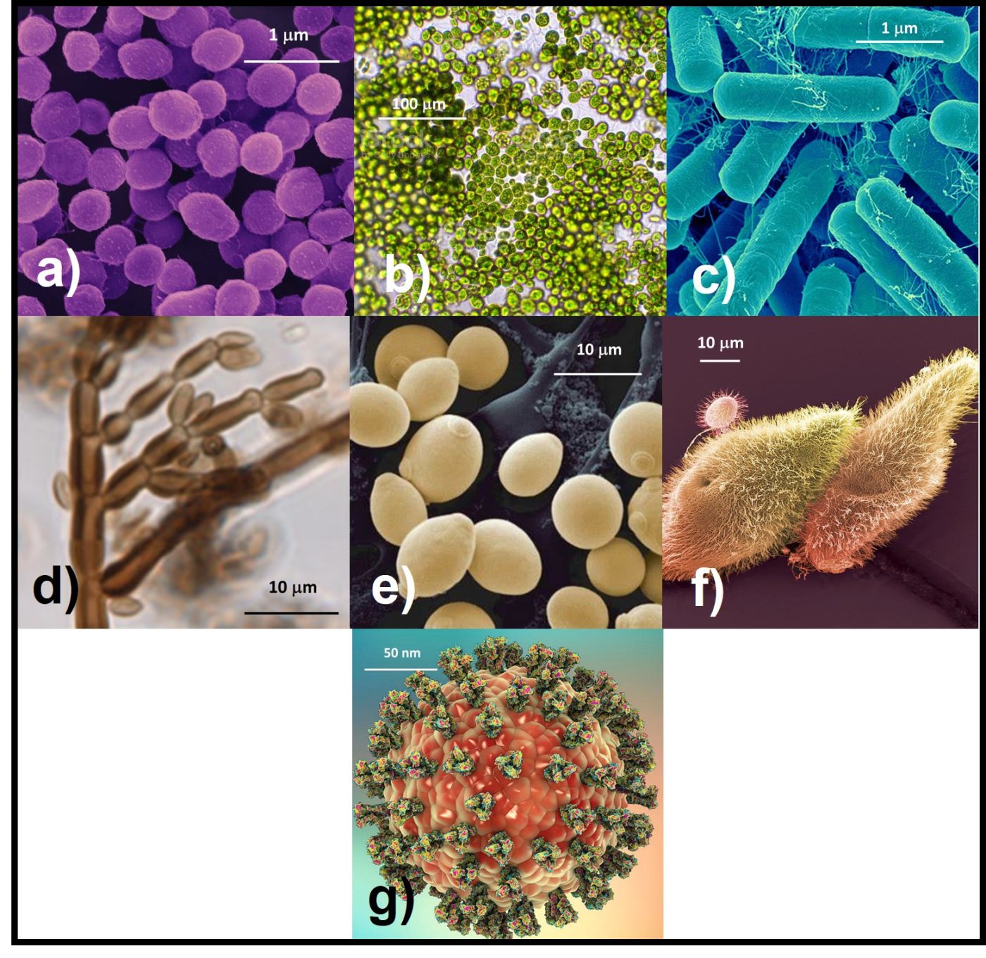
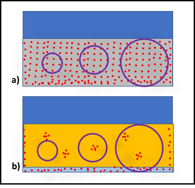
Dr. Jiri Snaidr of Vermicon AG (Hallbergmoos, Germany) reported on the development of a gene probe system for detecting specific microbes in fuel systems. The prototype flow cytometry system relied on fluorescent dye linked, ribonucleic acid (RNA) to label target microbes. After specimens are stained, they are drawn through a flow cytometer. Each target microbe is stained with a dye that fluoresces at a different wavelength so that the abundance of each organism can be quantified. Over the past decade, a new generation of flow cytometer has been developed that has made the technology an increasingly useful tool for quantifying microbial contamination in liquids. There are several challenges related to the use of flow cytometry for microbial contamination in fuels. As I’ll discuss below, the variety of microbes and types that exist in different fuel systems is considerable. Probes designed to detect specific microbes are likely to miss others that might be present. Additionally, microbial population densities in fuel samples is likely to be <1 cells mL^-1 . This means that in order to reliably detect fuel contaminant microbes, specimens will need to be ≥1 L.

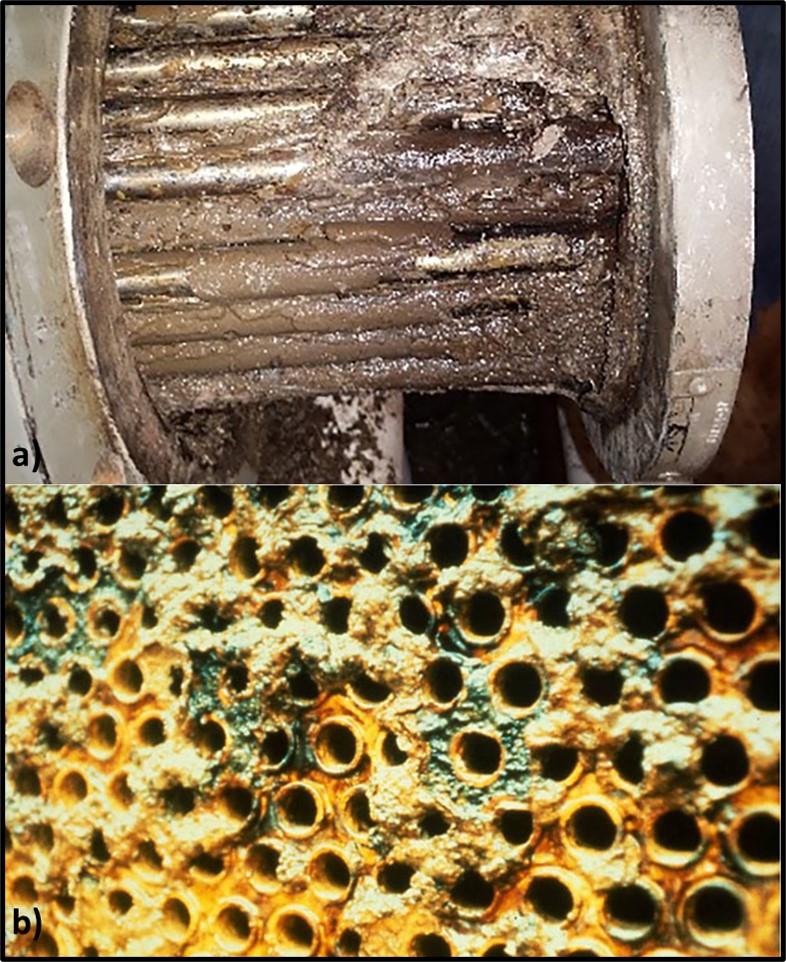
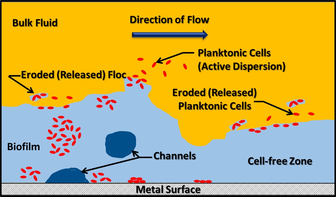
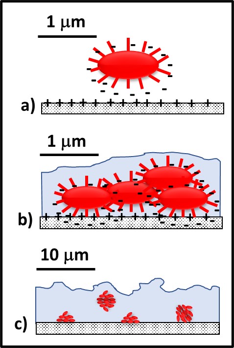
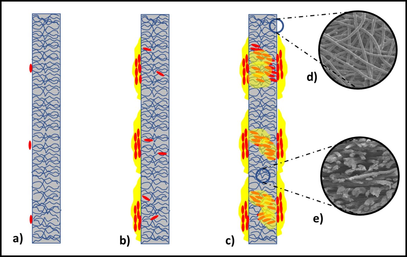
Dr. Osman Radwan of University of Dayton Research Institute (Dayton, OH, USA) discussed the use of an electrochemical biosensor to detect biofilm development on fuel system surfaces. Dr. Radwan’s multi-phase, fluidic device is comprised of an array that is pretreated with a protein molecule believed to be universally present among fuel degrading fungi (i.e., a biorecognition element – BRE). When microbes are bound to the protein, they generate an electrochemical signal. To date, Dr. Radwan and his colleagues have performed in-lab tests demonstrating their ability to detect filamentous fungi and single-cell yeasts. One challenge common among devices such as the one that Dr., Radwan described is that the sensor quickly becomes saturated. The sensors detect initial biofilm formation but cannot differentiate between a 10 µm or 1,000 µm thick film. It is generally recognized that fuel and fuel system biodeterioration are primarily due to the activities of biofilm communities. Thus, being able to assess three-dimensional biofilm growth is an important requirement for surface sensor arrays. Both Dr. Snadir and Dr. Radwan presented cutting edge technologies that are likely to take years of further development before they will be ready for commercial deployment, but their work is exciting and points towards the future.

Biodeterioration Mitigation and Contamination Control

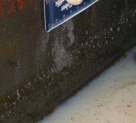
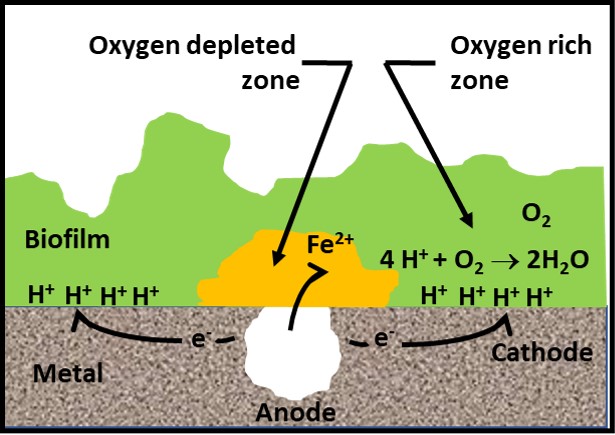
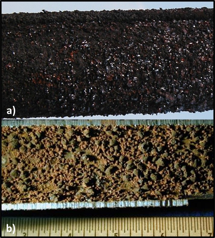
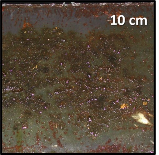
Graham Hill, of ECHA Microbiology, Ltd. (Cardiff, Wales, UK) discussed the relationship between salinity and sulfate reducing bacterial (SRB) activity in marine, seawater ballasted, fuel tanks. Microbiologically influenced corrosion (MIC) has been a problem in ships’ fuel tanks since the early 20th century transition from coal to liquid fuels. In order to maintain stability, ships take on seawater as they consume fuel. One of the most serious, unintended consequences of sea water ballasting is that the combination of seawater and fuel create an excellent environment for the proliferation of microbes. Aerobic and facultatively anaerobic microbes scavenge oxygen and produce low molecular weight organic acids on which SRB can thrive. Mr. Hill reported the results of lab-scale tests run at ECHA. His team found that by using freshwater, rather than seawater – i.e., keeping the salinity at <9 g L^-1 (the typical salinity of ocean water is 35 g L^-1) – reduces SRB activity (sulfate production) substantially.

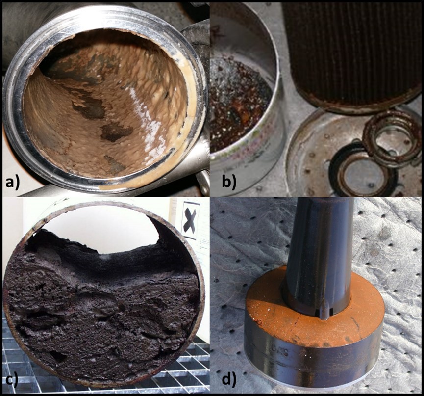
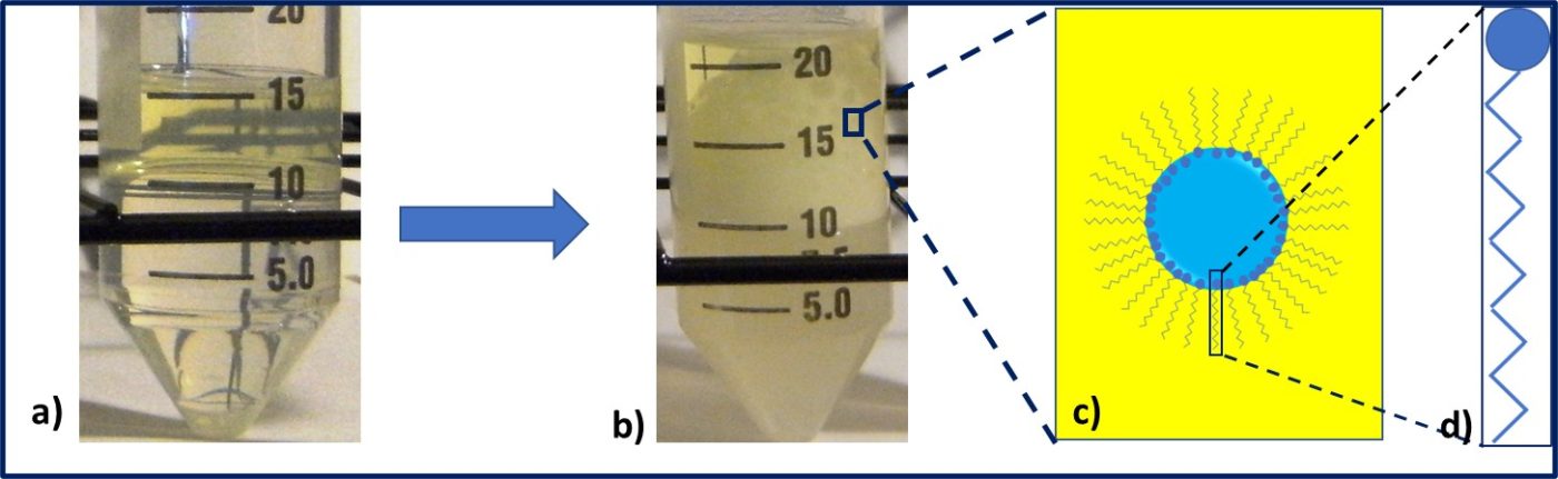
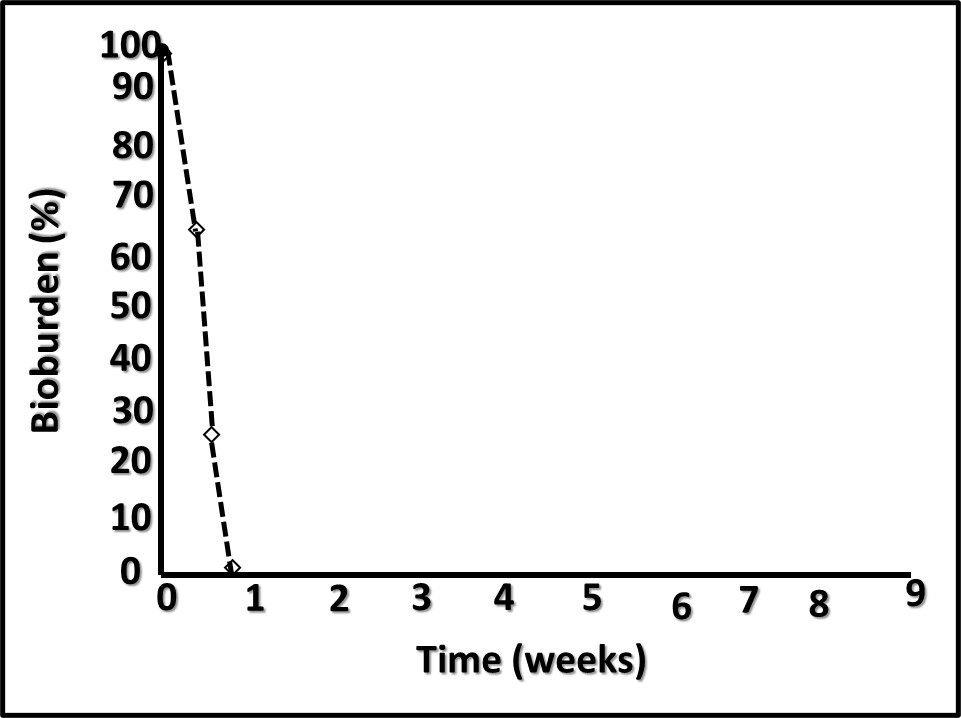
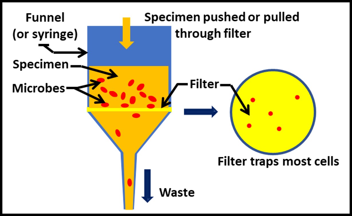
Dr. Oscar Ruiz, U.S. Air Force research Lab (AFRL, Dayton, OH, USA) reported on successful laboratory tests that demonstrated the efficacy of a graphene oxide (GO), nanoparticle, depth filter to scrub microbes from fuel. Dr. Ruiz report the results of a 227 m³ (60,000 gal) trial. At flow rates ≤ 40 L min^-1 (≤10 gpm) the device removed >90 % of the bioburden. At the end of the test the pressure differential across the filter was < 28 kPa (4 psi). Given the increased regulatory pressure against the use of fuel-treatment, antimicrobial pesticides (biocides), filtration is a promising alternative. Traditional filter media develop a cake that improves filtration efficacy to a point. Once the filter has accumulated too much material, pressure differentials increase, and flowrates decrease. If GO media can overcome this limitation, they might change the nature of fuel filtration. Filtration’s primary limitation is that the microbes that pass through the medium can colonize downstream surfaces and form biofilm communities. Filtration does not address biofilm control.

Microbial Ecology

Dr. Gareth Wiliams of ECHA Microbiology, Ltd. (Cardiff, Wales, UK) reported the results of an investigation into the factors contributing to hydrogen sulfide generation in salt caverns in which butane was stored. The ECHA team used quantitative polymerase chain reaction (qPCR) and next generation sequencing (NGS) to identify microbes in salt dome samples. Dr. Williams reported that of three caverns tested, hydrogen sulfide accumulated only in one. However, the microbial population profiles were similar among all three caverns. All three had SRB and Halobacterium species (Halobacterium is a genus within the domain of Archaea). The primary difference among the three caverns was the suction line installation. The cavern in which substantial concentrations of hydrogen sulfide had developed had an irregular floor. The uptake line was above the bottom; allowing brine to accumulate. The uptake lines in the other two caverns were at the bottom. In these caverns there was no bottom brine layer.

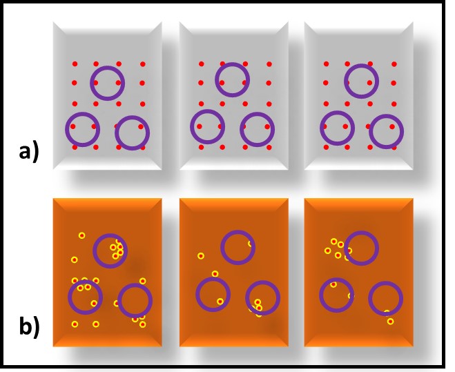
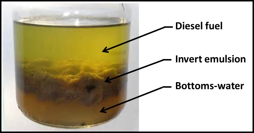
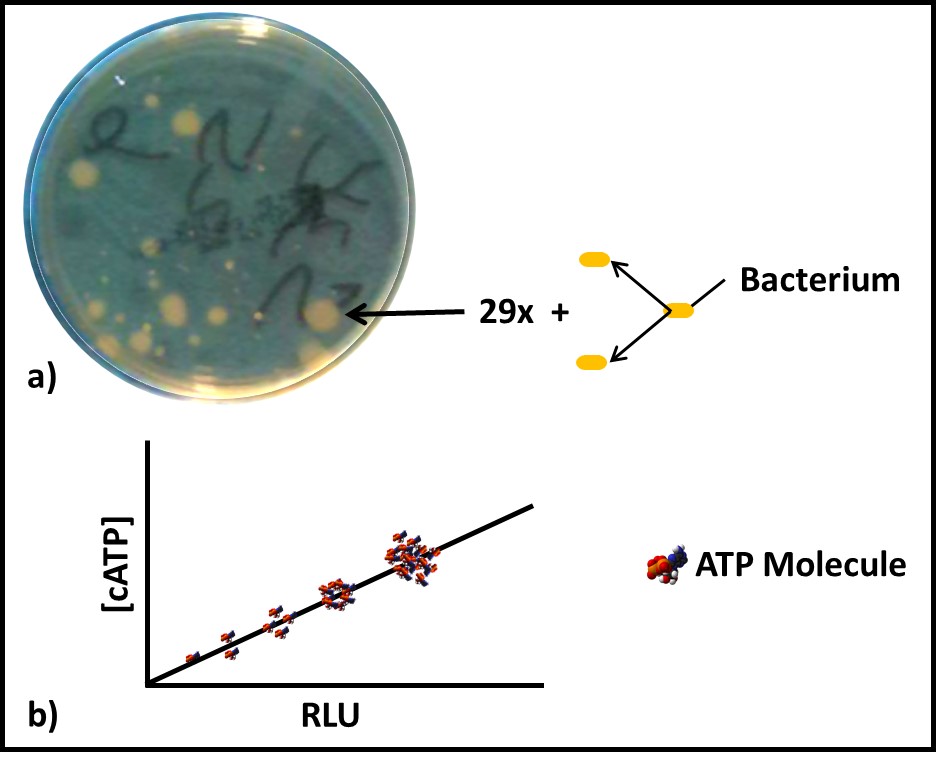
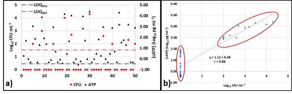
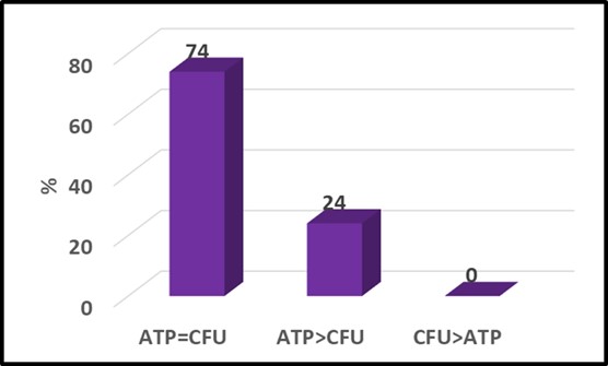
I presented NGS genomic data from the CRC-sponsored diesel fuel microcosm study from which I had reported adenosine triphosphate (ATP and adenylate energy charge (AEC) results at ICSHLF 16 in 2019 (The Relationship Between Planktonic and Sessile Mirobial Population Adenosine Triphosphate Bioburdens in Diesel Fuel Microcosms | IASH Online Library of Conference Proceedings and Newsletters (conferencespot.org) and The Relationship Microbial Community Vitality and ATP Bioburden in Bottoms Waters Under Fuel Microcosms | IASH Online Library of Conference Proceedings and Newsletters (conferencespot.org) – both are accessible to IASH members only. If you cannot access the papers, contact me for copies). Although during the original study (DP-07-16-01-FINAL-REPORT-REV-30JUL21-COMPLETE.pdf (crcao.org)) only a few aqueous phase samples were subjected to NGS testing. We were able to obtain the microcosms after 18-months. Marathon Petroleum, LuminUltra Technologies Ltd., and BCA collaborated to collect samples from the fuel-water interface and aqueous phases f 32 microcosms. LuminUltra Technologies Ltd. Performed the 18-month NGS tests and a different lab had performed the 3-month tests. Among the eight microcosms for which there were data from 3 and 18 months, the genomic profiles of four microcosms had remained stable and those of the other four changed substantially. Duplicate samples from several 18-month microcosms demonstrated that variability among duplicate aqueous samples was excellent but that variability among duplicate interface samples was substantial. Genomic test methods continue to evolve rapidly. As the protocols are refined, it will be essential to understand the sources of variation related to sampling and testing. Without this understanding, results from environmental samples will be difficult to interpret. I’ll devote a future What’s new post to genomics, transcriptomics, and metabolomics.

Lifetime Achievement Award

During the conference banquet I was taken totally by surprise when I was called to the stage to receive IASH’s Lifetime Achievement Award. I confess that when 1 st Vice-Chair, Matt DeWitt announced that it was time to present awards, I commented to my tablemates that these awards have never been given to microbiologists we are such a small minority within the Association. As I was making the comment, I heard my name. Did I mention that I was taken totally by surprise?

The award citation reads:

“By the members of IASH in recognition of his significant technical contributions and leadership related to testing, control and mitigation of microbiological contamination in fuels and oils. His notable technical contributions include over 70 technical publications on fuel, lubricant and metalworking fluid microbiology and biodeterioration. He has had numerous Chair and leadership positions in ASTM, IBBS, and IATA, and contributed significantly to the development of best industry practice documents and guidelines for the prevention and control of microbiological contamination in fuels.”

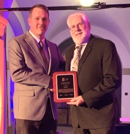
1st Vice-Chair Matt DeWitt presenting IASH Lifetime Achievement Award to Fred Passman

Summary

In summary, the conference was an exceptional opportunity to learn about various aspects of fuel degradability and its control. I most strongly recommend that individuals who are responsible for fuel quality join IASH and make plans to attend future IASH conferences. Again, for more information about IASH, visit Home (iash.net).

To contact me, please send an email to fredp@biodeterioration-control.com.

WHAT ARE BIOFILMS AND WHY DO THEY MATTER? PART 2 – BIOFILM-RELATED PROBLEMS

Biofilm at Metalworking Fluid Surface – Sump Wall Interface.

Biofilms Part 1 Recap

In my last What’s New article I wrote:

Biofilms can form on any surface that is in contact with water. In aqueous systems such as heat exchanger, potable water, firemain, containing water-miscible metalworking fluid, biofilms can coat >90 % of surfaces in contact with the fluid. In systems containing fuels, lubricants, or other fluids in which water is not normally miscible, biofilms typically develop in zones where condensate water accumulates.

Biofilms are complex structures comprised primarily of EPS. Microbes living in biofilm consortia resemble the cells of multicellular organisms. Physiologically, they can be quite distinct from genetically identical planktonic cells. Additionally, genetically identical microbes can differ physiologically based on their location within the EPS matrix. Due to the combined effects of microbial metabolic activity and EPS chemistry, the physicochemical environment within biofilms can be very different from that of the fluid with which it is in contact. Chemical gradients within biofilms contribute to microbiologically influenced corrosion (MIC).

In this article, I’ll review the types of biodeterioration damage that can be associated with biofilms. In particular, I’ll discuss:

• Biofouling
• Heat exchanger, heat transfer reduction
• Microbiologically influenced corrosion (MIC)

Biofouling

Biofouling is the unwanted accumulation of organisms, their excreted polymers (see EPS discussion in the May 2022 What’s New article), and entrained substances on surfaces. Although multicellular organisms, such as barnacles, can be part of biofouling communities, in this article I’ll focus on microbial biofouling. Figure 1 shows four examples of biofouling. Figure 1a is a fermentation unit’s transfer line. Biofouling contributes to finished product contamination and inhibits flow from the fermenter to the drying unit. Figure 1b is a fouled fuel dispenser filter element. This is the most common cause of reduced fuel flowrates at retail fuel dispensers (in the U.S., fuel should be dispensed at 10 gpm – 40 L min^-1; filter fouling can reduce the flowrate to <1 gpm – 4 L min^-1). In Figure 1c, biofouling has glued small metal particles (swarf) together in a metalworking fluid (MWF) return line. Swarf is generated during metal removal by grinding. In this pipe, EPS has glued the swarf particles into a solid mass, causing what I call industrial atherosclerosis (atherosclerosis is condition where the arteries become narrowed and hardened due to buildup of fats in the artery wall; industrial atherosclerosis occurs when biofouling narrows the internal diameter of a pipe).

Figure 1d shows biofouling on the surface of an automatic tank gauge’s (ATG’s) water float. In fuel storage tanks, ATGs are used to record both product and bottoms-water volumes. An ATG has two floats that move along a metal shaft. One float (not shown) is designed to rest on top of the fuel’s surface – signaling the total fluid volume in the tank. The water float’s specific gravity (SG) is greater than that of the fuel product, but less than that of water. Consequently, it rests at the fuel-water interface. Biofouling on the water float’s surface can either decrease or increase the float’s SG. If the biofilm has numerous gas pockets, it will decrease the float’s SG and cause it to register the presence of water even when none is present. If the biofilm is loaded with rust particles, it will increase the float’s SG. The float will fail to lift off the tank’s floor when bottom-water is present.

Fig 1. Biofouling – a) Fermenter transfer line; b) fuel dispenser filter; c) MWF used fluid transfer line; d) underground storage tank ATG water float.

In general terms, these four photographs illustrate how biofouling can affect industrial systems. Biofilm microbes on pipe surfaces can contaminate fluids as they flow through the line. Biomass accumulations on filter media can block fluid flow. Biofilm accumulation and the interaction between biofilm polymers and metal fines can restrict fluid flow by reducing the pipe’s functional inner diameter. Biofouling on sensor surfaces can cause sensors to generate inaccurate signals.

Although the next two biofilm-related problems depend on the presence of biofouling, the mere physical presence of biofilms can degrade industrial system operations. Think of this as passive biodeterioration – microbes are not attacking surfaces.

Heat exchanger, heat exchange inhibition

Biofilms are excellent insulators. One report (Biofilm effects on heat transfer of heat exchangers) estimated that a 5 µm thick biofilm can reduce heat exchange across copper tubes, in tube-in-shell heat exchangers, by 67 %. Tube-in-shell heat exchangers are fabricated by placing a tube bundle (Figure 2a) into an outer shell (Figure 2b). The water to be cooled either flows through the outer shell and the cooling water flows through the tubes or the cooling water flows through the outer shell and the water to be cooled flows through the tubes. Either way, the tremendous surface area to volume ratio facilitates heat transfer from the warmer fluid to the cooler fluid. The tubes are commonly made of aluminum, brass, copper, carbon steel, or stainless steel, although other metals are also used. Figures 3a and 3b respectively show heat exchanger biofouling on the exterior and interior tube surfaces. The heavy biofilms depicted in these photographs can reduce heat transfer by > 90 %.

Fig 2. A tube-in-shell heat exchanger – a) tube bundle; b) outer shell.

Thermal conductivity (λ) – expressed as W (m . K)^-1, where W is watts, m is meters, and K is temperature in degrees Kelvin – is a measure of the ease with which heat is transmitted through a material. Table 1 provides a list the λ-values for common heat exchanger tube and insulating materials. Although λ is important, other factors such as corrosion and scaling resistance, and durability are considered when selecting heat exchanger materials. Note that λ_biofilm is comparable to λ_{dry soil} and λ_water. All are excellent insulators.

A case study, reporting the impact of a 1 mm of biofilm in a 200-ton centrifugal chiller operating at 50% load, stated that heat exchange was reduced by 35 %.

Fig 3. A tube-in-shell heat exchanger – a) biofouling coating tube exterior surfaces; b) biofouling coating tube interior surfaces.

As with biofouling as a general category, biofilm functionality as an insulator is a physical phenomenon – independent of microbial metabolism within the biofilm matrix.

Microbiologically influenced corrosion

Microbiologically influenced corrosion (MIC) is the biologically mediated deterioration of a material. I’ll provide a more detailed discussion of MIC in a future What’s New article. For now, I will note that MIC occurs under biofilms. Globally, MIC causes an estimated $40 billion and $100 billion U.S. damage annually. As I explained in my May 2022 article, the biofilm creates electropotential gradients including zones in which oxygen (O₂) is relatively depleted. A Galvanic cell is an electrochemical cell in which an electric current is generated from oxidation-reduction reactions. The oxygen gradients within biofilms drive Galvanic oxidation-reduction reactions. As illustrated in Figure 4, an anodic cell forms under the oxygen depleted zone. Metallic iron (Fe) dissolves as ferrous iron (Fe²⁺) and electrons (e^–) flow towards the cathodic cell (metal under more oxygen rich zones within the biofilm). Although the cathode attracts hydrogen ions (H⁺), dissolve oxygen (O₂) can react with the hydrogen to produce water (H₂O). Hydrogen removal from the cathode propagates continued electron flow and metal dissolution.

Fig 4. Galvanic corrosion under biofilm.

Galvanic corrosion can occur without direct microbial involvement, although EPS production and aerobic respiration both contribute to creating the oxygen concentration differentials illustrated in Figure 4. In fuel over water systems, biofilm accumulation is typically heaviest at the fuel-water interface (Figure 5a). The corrosion coupon shown in Figures 5a (before biofilm removal) and 5b (after coupon was cleaned for corrosion analysis) was suspended in a jar that contained diesel fuel over an aqueous salts- solution. Note that the amount of damage to the coupon was also at the interface. Although MIC tubercles can be seen on the coupon’s surface in both the interface (Figure 5c) and aqueous (Figure 5d) contact zones, the number of tubercles per cm² is considerably greater in the interface zone. Similarly, as shown in the title photo, heaviest biofilm accumulation in MWF sumps tends to be found at the MWF-air-tank wall interface. MIC can also occur one surfaces exposed to water vapor or mist. In ships tanks, the heaviest corrosion is commonly observed on the tank overhead surfaces where water vapor condenses – providing an ideal habitat for fungal growth.

In metalworking facilities with central MWF systems, MWF returning from machines to filtration units flows through sluices. Historically, these sluices were covered with open grates. In the late 1990s grates were replaced by solid steel plates to reduce mist concentrations in facilities’ breathing zones (i.e., 1m to 2 m above the floor). This change effectively prevented mists generated in the sluice from escaping but provides a surface on which biofilms and MIC could develop (Figure 6).

Fig 5. Corrosion coupon from fuel over water microcosm – a) biofilm-coated coupon; b) coupon after cleaning; c) scanning electron microscope (SEM) image of coupon surface at fuel-water interface (inset circle is the area analyzed by energy dispersive x-ray analysis; d) SEM image of coupon surface in zone exposed to aqueous phase.

Fig 6. MWF return sluice deck plate (cover); underside.

Although biofilms and MIC develop only develop when sufficient water is present, Figure 7 illustrates how undetectable trace concentrations of water are sufficient to support MIC. Figures 7a and &b, respectively, show the exterior and interior surfaces of an UST’s submerged turbine pump’s riser. Nominally, these surfaces are in contact only with fuel. However, the exterior corrosion and innumerable tubercles on the interior surface would not have formed had they not been exposed to sufficient free water to support microbial growth.

Fig 7. UST submerged turbine pump riser pipe – a) exterior surface; b) interior surface after pipe was cut in half, longitudinally.

Galvanic corrosion is only one of several MIC mechanisms. Surface depassivation (H⁺ ion removal) was the first MIC mechanism described. Passivation – the arrest of electron flow in a galvanic cell – occurs when the H⁺ ions accumulating on the cathode for a film. As part of the sulfate reduction pathway, sulfate reducing bacteria (SRB) scavenge hydrogen from a galvanic cell’s cathode. This depassivates the surface – accelerating electron flow and metal dissolution. This mechanism was reported in the 1940s before microbiologists recognized the significance of biofilms. Although SRBs are still considered to play a significant MIC role, since the 1970s it has become apparent that low molecular weight (primarily C₁ – formic, C₂ – acetic, and C₃ – lactic acids) organic acids (LMWOA) produced by all microbes contribute to MIC. These LMWOA can react directly with metal surfaces or can react with dissolve inorganic salts such as sodium or calcium chloride to form a strong inorganic acid (hydrochloric acid – HCl) and a weak organic base (the sodium C₁, C₂, or C₃ salt – sodium formate, sodium acetate, or sodium lactate). Strong acids such as HCl can dissolve metals aggressively. Because biofilms act as barriers, the concentration of acids at the biofilm-metal surface can quite high (e.g., 1N hydrochloric acid, 2N sulfuric acid, etc.). The pH in this high acid zone can be <2. Aggressive MIC under a biofilm can drill a hole in 1 cm think mild steel pipe or tank walls in less than six months.

Summary

Biofilms primarily contribute to three types of biodeterioration: biofouling, insulation, and corrosion. When a biofilm is present, all three types of biodeterioration can be occurring simultaneously. By creating a barrier between sensors and fluids, biofilms can cause sensor failures. Heavy biofilm accumulations can restrict fluid flow through pipes. Even thin (<5 µm) biofilms can substantially reduce heat transfer in heat exchangers. Ineffective heat exchange causes process fluid overheating and consequent fluid, system or both types of failure. MIC occurs under biofilms. Combined, these biodeterioration mechanisms cause more than $100 billion U.S. annual damage globally.

In my next What’s New article I’ll discuss general approaches for biofilm control. In the meantime, if you have any questions about the information in this post, don’t hesitate to contact me at fredp@biodeterioration-control.com.

WHAT ARE BIOFILMS AND WHY DO THEY MATTER? PART 1 – BIOFILM FOUNDATIONS

Metalworking fluid return sluice cover plate; underside, showing biofilm build-up.

What are biofilms?

ASTM¹ defines biofilm as a noun: “microorganisms living in a self-organized community attached to surfaces, interfaces, or each other, embedded in a matrix of extracellular polymeric substances of microbial origin, while exhibiting altered phenotypes with respect to growth rate and gene transcription.” The ASTM definition adds: “Biofilms may be comprised of bacteria, fungi, algae, protozoa, viruses, or infinite combinations of these microorganisms. The qualitative characteristics of a biofilm, including, but not limited to, population density, taxonomic diversity, thickness, chemical gradients, chemical composition, consistency, and other materials in the matrix that are not produced by the biofilm microorganisms, are controlled by the physiochemical environment in which it exists.”

There are quite a few complex terms used in this definition. In today’s article, I’ll unpack the definition and explain why people involved with industrial fluid or system management should pay attention to biofilms.

Microorganisms

If you have been reading my What’s New articles, you already know what microorganisms are. They are organisms that are too small to be seen without the use of a magnifying device such as a microscope (Figure 1). Here’s a quick refresher (all definitions are for plural terms and are quotes from ASTM terminology standards):

• Algae – major group of lower plants, generally aquatic, photosynthetic of extremely varied morphology and physiology, monocellular plants with chlorophyll often masked by a brown or red pigment.
• Archaea – (domain Archaea), any of a group of single-celled prokaryotic organisms (that is, organisms whose cells lack a defined nucleus) that have distinct molecular characteristics separating them from bacteria (the other, more prominent group of prokaryotes) as well as from eukaryotes (organisms, including plants and animals, whose cells contain a defined nucleus).
• Bacteria – any of a class of microscopic single-celled organisms reproducing by fission or by spores. Characterized by round, rod-like, spiral, or filamentous bodies, often aggregated into colonies or mobile by means of flagella. Widely dispersed in soil, water, organic matter, and the bodies of plants and animals. Either autotrophic (self-sustaining, self-generative), saprophytic (derives nutrition from nonliving organic material already present in the environment), or parasitic (deriving nutrition from another living organism). Often symbiotic (advantageous) in man, but sometimes pathogenic.
• Fungi – single cell (yeasts) or filamentous (molds) microorganisms that share the property of having the true intracellular membranes (organelles) that characterize all higher life forms (Eukaryotes).
• Protozoa – a phylum or group of phyla that comprises the single-celled microscopic animals, which include amoebas, flagellates, ciliates, sporozoans, and many other forms.
• Virus – an infective agent that typically consists of a nucleic acid molecule in a protein coat, is too small to be seen by light microscopy, and is able to multiply only within the living cells of a host.

Fig 1. Microorganisms – a) archaea; b) algae; c) bacteria; d) fungi – molds; e) fungi – yeasts; f) protozoa; g) virus. Note size ranges from viruses (150 to 200 nm dia) to algae (100 µm dia).

Self-organized community

A self-organized community is one that forms due to the activities of its members. As I’ll explain in more detail below, biofilms are complex creations that are quite similar to multi-cellular organisms such as sponges and all higher organisms. The shape and function of each cell within the biofilm matrix is affected by chemical signals it receives from other cells.

Matrix of extracellular polymeric substances of microbial origin

A matrix is the set of conditions that provides a system in which something grows or develops. A biofilm matrix is a complex mixture of biomolecules, including genetic material (deoxyribonucleic acid – DNA – and ribonucleic acid – RNA), peptides, lipids, carbohydrates, and other large molecular weight molecules. This mixture is called extracellular polymeric substance (EPS). Originally (when I was an undergraduate investigating biofilm development on cave steam surfaces) biofilms were thought to be homogeneous surface coatings – not unlike a uniform layer of slimy paint. Now we understand that the EPS matrix is structurally complex. As Figure 2 illustrates, within the biofilm’s EPS matrix there are cell-dense and cell-free zones. Additionally, channels provide for nutrient and metabolite flow within the biofilm. Biofilms release cells into the bulk fluid by two mechanisms. Passive release occurs due to the erosive effects of fluid flowing over the biofilm. However, biofilm communities can also release cells actively. Planktonic microbes released from biofilms can settle on downstream surfaces and pioneer the creation of new biofilm communities. Some zones within the biofilm are tightly packed with microbial cells and others are cell deserts – with no cells visibly present.

Fig 2. Biofilm schematic. Red shapes of microbial cells. Light blue area is the EPS. Dark blue areas are channels, and yellow area is the bulk fluid flowing over he biofilm.

The process of biofilm development has been well studied. Bacteria with specialized external structures called attachment pili are attracted to substrate surfaces (for example, metal or concrete surfaces) by electrostatic and other forces (Figure 3a). This is called the attachment phase, or Stage I, of biofilm development. During Stage II (the growth phase), these pioneering bacteria replicate and start producing EPS (Figure 3b). In many environments, a mature biofilm (Stage III; Figures 2 and 3c) can develop within 24 h to 72 h. The population in a mature biofilm can consist of a single type of microbe (operational taxonomic unit – OTU – or genotype), when the microbes in the EPS matrix are genetically identical (i.e., monoclonal), or diverse OTUs.

Fig 3. Biofilm development – a) pioneer bacteria with attachment pili are attracted to surfaces by various electrochemical forces; b) after attaching to surfaces, pioneer bacteria reproduce, and excrete adhesive polymers and EPS; c) with a few days, the mature biofilm has formed.

Microbes within the biofilm form a consortium. They signal to one another by secreting and sensing various types of biomolecules. This molecular communication among cells is quite sophisticated and resembles the kind of intercellular communication that takes place among cells in multicellular organisms ranging from sponges to humans.

Phenotype

A phenotype is a set of an organism’s observable characteristics resulting from its interaction of its genotype with the environment. Just as the appearance and function of human cells depend on their location (e.g., skin cells, liver cells, muscle cells, etc. – all of which vary based on the organ of which they are part and their location within the organ – think of the many different cell phenotypes in an eyeball!), the appearance and function of microbial cells can vary with their immediate environment. Nearly 20 years ago, researchers at the Montana State University’s Center for Biofilm Engineering (Center for Biofilm Engineering – Center for Biofilm Engineering | Montana State University) placed a single bacterial cell onto a glass surface and watched as it reproduced and created a biofilm consortium. The researchers found that both the shape (morphology) and physiological characteristics (nutrients the cell can consume and waste products it excretes) of a single genotype depended on cells’ locations within the biofilm matrix. Reiterating my earlier comment: think of biofilm consortia as being among the earliest multicellular organisms. It is likely that early reports of biofilm microbial diversity included incorrect assessments based on phenotypic differentiation among cells. The biofilm literature now includes descriptions of both monoclonal and genetically diverse biofilm consortia.

Genetic Transfers

Confused yet? Microbes living in close proximity are exceptionally promiscuous. They can exchange both chromosomal and extrachromosomal DNA. Chromosomal DNA is the DNA contained in the threadlike structure that contains the organism’s genes which, in turn, define its genotype. Plasmids are strands of DNA that are not part of a cell’s chromosome. Plasmids can replicate independently of the chromosome. They can be present inside cells or in the EPS matrix. When plasmids from the environment enter cells, the process is called transfection.

Bacterial can transfer both chromosomal DNA and plasmids through conjugation pili. This process is called conjugation. Figure 4 illustrates the conjugation process. After the plasmid replicates inside one cell (Figures 1a and 1b), it can be transferred via a conjugation pilus (singular form of pili) to another cell (Figures 1c, through 1e). At the end of the process, both sells have the plasmid (Figure 1f). Plasmids are an essential tool for genetic engineering. In nature, they are the primary means by which properties such as microbicide resistance are transferred among cells.

Fig 4. Plasmid gene transfer by conjugation – a) two bacterial cells – one with and one without the plasmid; b) plasmid replicates; c) conjugation pilus connects two cells; d) plasmid DNA enters conjugation pilus for transfer to recipient cell; e) plasmid transfer has completed; f) both cells can now transfer plasmid to other cells.

Bacterial and fungal viruses can also act as vectors for gene transfers. When a DNA virus infects a host cell, its DNA is typically integrated into the host cell’s chromosome. As new viruses are produced within the host cell, some of the virions can pick up one or more genes from the host’s chromosome. After the host cell lyses, the released virions attach to new host cells. Those carrying genes from the previous host cell can transfer those genes to their new hosts. This process is call transduction.

Gene transfer among biofilm consortium cells is one of several communications mechanisms. Additionally, it is a process that spreads adventitious genes (such as microbicide resistance) among members of the biofilm community.

Summary

Biofilms can form on any surface that is in contact with water. In aqueous systems such as heat exchanger, potable water, firemain, containing water-miscible metalworking fluid, biofilms can coat >90 % of surfaces in contact with the fluid. In systems containing fuels, lubricants, or other fluids in which water is not normally miscible, biofilms typically develop in zones where condensate water accumulates.

Biofilms are complex structures comprised primarily of EPS. Microbes living in biofilm consortia resemble the cells of multicellular organisms. Physiologically, they can be quite distinct from genetically identical planktonic cells. Additionally, genetically identical microbes can differ physiologically based on their location within the EPS matrix. Due to the combined effects of microbial metabolic activity and EPS chemistry, the physicochemical environment within biofilms can be very different from that of the fluid with which it is in contact. Chemical gradients within biofilms contribute to microbiologically influenced corrosion (MIC).

My next What’s New article will expand on how biofilms contribute to biodeterioration problems. In the meantime, if you have any questions about the information in this post, don’t hesitate to contact me at fredp@biodeterioration-control.com.

¹ ASTM E2196 Standard Test Method for Quantification of Pseudomonas aeruginosa Biofilm Grown with Medium Shear and Continuous Flow Using Rotating Disk Reactor, https://www.astm.org/e2196-17.html.

MIRCROBIAL CONTAMINATION IN TURBINE OIL SYSTEMS? ARE YOU KIDDING!?

Microbes do not care whether operators accept the science.

Can microbes degrade turbine oil and cause damage to turbine oil systems?

The short answer is yes.

In 2018, as part of an Energy Institute sponsored project, I invited more than 100 turbine system operators to complete a survey designed to assess biodeterioration risk awareness and operational measures (for example, condition monitoring practices) for reducing the risk. Concurrently, I sent a similar invitation to power generation facility operators responsible for emergency standby diesel generator fuel systems. In contrast to the 23 % response from the folks responsible for fuel systems, I received no complete responses from folks responsible for turbine oil systems. Clearly, personnel responsible for fuel systems were more aware of the risk of biodeterioration than were their colleagues responsible for turbine oil systems.

Turbine oil and turbine oil system biodeterioration is not a common occurrence, but it does happen. A major challenge is that the people who need to connect the dots, are typically unaware of the potential for microbes to grow in these systems.

In this What’s New article I will summarize thet types of damage microbes can cause to turbine oil systems when sufficient water is present.

Water

Although microbes require free water (water that has coalesced into droplets or a continuous phase) the volume they require can be vanishingly small. In my education courses, I compare a 1 µm (0.000039 in) bacterium on a surface under a 1 mm (0.039 in) film of water (Figure 1a) to a 2 m (6ft) tall person standing on the floor of a lake that is as deep as Mt. Kilimanjaro is tall (6,000m – 20,000 ft – Figures 1b and 1c). Moreover, a one mL (0.034 oz) drop of water can be a habitat for more than a billion bacterial cells. Thus, undetectably small traces of water can support substantial microbial communities and those communities can degrade the oil and damage the turbine oil system. Note: this phenomenon applies equally traces of water found in fuel and hydraulic fluid systems.

Fig 1. Relativity – the environment provided by a 1 mm thick film of water – a) relative dimensions of a 1 µm -long bacterium in 1 mm of water in graduated cylinder; b) a 2 m tall person standing at the base of Mt. Kilimanjaro; c) the same person standing on the floor of a lake that is as deep as Mt. Kilimanjaro is tall.

The most common symptom of uncontrolled microbial contamination in turbine oils is increased entrained water as determined by the Karl Fischer test (ASTM Test Methods D1533 or D6304). Water’s solubility in turbine oils can range from 20 µg kg^-1 (i.e., ppt) to 60 µg kg^-1. Optimally, it is maintained at <50 µg kg^-1. Figure 2, copied from an article in Machinery Lubrication, shows that petroleum based turbine oils typically become visibly hazy once the water concentration reaches approximately 100 µg kg^-1 (0.1 %). The water solubility in phosphate ester (PE) based oils is approximately 10x greater (i.e., 1,000 µg g^-1). Haze (cloudiness) indicates that the concentration of water in the oil has exceeded its solubility and that the water has coalesced into micelles (droplets). Figure 3a shows oil in which the water concentration is below the saturation concentration. Figures 3b and 3c show how increased volumes of dispersed water increase the oil’s haziness; ultimately forming an invert emulsion.

Fig 2. Relationship between water concentration and haze (and bearing life).
Source: Water In Oil Contamination (machinerylubrication.com)

Fig 3. Relationship between water concentration and haze – a) water concentration is below the saturation level – the oil is clear and bright; b) water concentration is greater than saturation level – the oil has become hazy; c) sufficient water is present to form an invert emulsion.

What does this have to do with microbes? Microbes can produce detergent-like molecules called biosurfactants. As illustrated in Figure 4, biosurfactant molecules create stable, invert (water-in-oil) emulsions. Invert emulsion micelles provide oil-water surface area that facilitates microbes’ ability to use base-stock and additives as food.

Fig 4. Biosurfactant-based, invert emulsion – a) oil over water that is infected with biosurfactant—producing microbes; b) sample show in (a), 30 min after vigorous shaking – note formation of a stable, invert-emulsion; c) invert emulsion – water droplet encased by biosurfactant molecules; d) biosurfactant molecule showing polar (charged) head and non-polar (chargeless, hydrocarbon) tail.

Thus, water provides an environment in microbes can thrive. Thriving microbes produce biosurfactants that degrade the oils water separability properties (ASTM Test Method D1401) and thereby make nutrients from oil more readily available to the infecting microbes. Now I’ll summarize the primary consequences of providing microbes with the water they need to thrive.

What damage can microbes cause to turbine oils?

The process by which microbes (and all other living things) consume nutrients and convert them into food, energy, and waster is called metabolism. Microbes can directly consume oil additives, including corrosion inhibitors, antioxidants, and lubricity additives. They can also consume base oils. The net effect of this metabolic activity includes:

• Decreased base number
• Decreased oxidative stability
• Decreased water separability (as noted above)
• Decreased corrosion inhibition
• Increased acid number
• Increased particle load
• Increased water content (as noted above)
• Degraded viscosity and viscosity index properties

You’ll probably notice that each of these symptoms of turbine oil degradation can also be caused by non-microbiological (abiotic) processes. That creates a significant challenge when attempting to distinguish between biodeterioration and abiotic deterioration. More on that below.

What damage can microbes cause to turbine oil systems?

Premature filter plugging

In Figure 5, the oil is flowing from left to right. Unlike organic and inorganic particles, when microbes are trapped onto filter surfaces (Figure 5a) they can reproduce (proliferate) and excrete extracellular polymeric substance (EPS – a blend of various macromolecules that includes lipids, carbohydrates, proteins, nucleic acids, and others). Consequently, filter media are coated with both an increasing mass of cells and EPS (Figure 5b). Microbes trapped within the filter’s matrix can also proliferate and produce EPS. The combination effect is premature filter plugging as indicated by an increased pressure differential across the filter (Figure 5c). Figures 5d and 5e are photomicrographs of a filter’s surface and cross-section – illustrating how the weaved fibers achieve the medium’s designated porosity and filtration efficiency.

Fig 5. Microbes causing premature filter plugging- a) microbes (bacteria) trapped on upstream side of filter; b) trapped microbes proliferate and produce EPS; c) microbial colonization and EPS production no and within matrix restricts oil flow – causing high pressure differential across filter; d) inset showing surface view of filter’s fibers; e) inset showing cross-section view of filter’s fibers.

Corrosion

Microbiologically influenced corrosion (MIC) is an umbrella term that includes direct and indirect mechanisms by which microbes contribute to corrosion. I’ll devote a future What’s New article to explaining MIC. For now, I’ll simply note that MIC most commonly contributes to failures of pressurized lines and that (have you read this before?) MIC shares symptoms with abiotic corrosion mechanisms.

Reservoir fouling

Figures 3 and 4 illustrate mild forms of invert emulsion. Figure 6 is a sample from the bottom of a turbine oil reservoir. The invert emulsion residue that was produced by microbes in the system was nearly solid. To remove it from the reservoir, operators had to drain the tank, shovel out the semi-sold mass from the bottom 5 cm (2 in), then use high pressure, hot water and detergent to clean the reservoir before retuning it to service. Lines in which this mass had congealed had to be replaced.

Fig 6. Turbine oil reservoir bottom sample showing 5 cm layer of semi-solid, invert emulsion associated with uncontrolled microbial contamination.

Summary

When sufficient water to present, microbes can proliferate and be metabolically active in turbine oil systems. When this happens, microbial populations can degrade both the oil and the system. For a full treatment of the problem and its mitigation, read Energy Institute’s Guidelines on detecting, controlling, and mitigating microbial growth in oils and fuels used at power generation facilities, 1 st Ed., June 2020, ISBN 978 1 78725 188 5 (Figure 7).

Fig 7. Cover – EI Guidelines on detecting, controlling, and mitigating microbial growth in oils and fuels used at power generation facilities, 2020.

As always, I look forward to receiving your questions and comments at fredp@biodeterioration-control.com.

WHAT CONTRIBUTES TO MICROBIOLOGICAL TEST RESULT VARIABILITY?

Sources of Variation. Homogeneity – the non-uniform distribution of microbes in the sample source (V_SOURCE, where V = variability), the sample (V_SAMPLE) and the specimen (V_SPECIMEN) – contributes substantially to test result variability.

It’s Not the Method

A few years ago, a single set of fuel and fuel-associated water samples were used for two ASTM interlaboratory studies (ILS). You can read the details in the paper published in International Biodeterioration & Biodegradation. The ILS were performed based on the guidance provided by ASTM Practice D6300 for Determination of Precision and Bias Data for Use in Test Methods for Petroleum Products, Liquid Fuels, and Lubricants. As we discovered, D6300 is only applicable to properties that are both homogeneous and stable. Microbial contamination is neither. The two ILS were for ASTM Methods D7687 for Measurement of Cellular Adenosine Triphosphate in Fuel and Fuel-associated Water With Sample Concentration by Filtration and D8070 for Screening of Fuels and Fuel Associated Aqueous Specimens for Microbial Contamination by Lateral Flow Immunoassay. A few hours before the first ILS, specimens were prepared from samples known to have high, intermediate, and low bioburdens. Per D6300 a specimen was 200 mL fluid in a container, with three replicate containers for each combination of samples type (fuel grade or bottoms-water) and bioburden. Each container received a randomized code so that ILS participants would not know its contents. Preliminary ILS indicated that repeatability (single analyst) variability was < 5 % for each of the methods. Shockingly, the data from the D6300-based ILS indicated that both repeatability and reproducibility variability for each method were astronomical. I use the word shocking because both methods had long histories of yielding precise test results. The results suggested that the bioburdens in supposedly identical, replicate samples were actually substantially different. To test this theory, my collaborators and I compared the D7687 and D8070 results for each specimen. We found result agreement for 108 of 128 specimens (84 % agreement between methods). These findings inspired the development of ASTM Guide D7847 for Interlaboratory Studies for Microbiological Test Methods. The Guide enables ILS planners to reduce the variability of bioburdens in specimens so that test method rather than bioburden variability is tested.

In today’s What’s New article, I’ll explain some of the factors that contribute to test result variability. Remember that it is essential to understand test method variability before attempting to set data-based control limits.

Microbiological Test Result Variability – Are Microbes Present?

Are samples collected from locations most likely to have microbes?

In July 2021’s What’s New article, I wrote that the variability of microbiological test data is substantially greater than for other of tests used to analyze fuels, hydraulic fluids, lubricants, metalworking fluids (MWF), and other fluid samples. The non-uniform (heterogeneous) distribution of microbes in these fluids is often the primary factor contributing to test result variability.

The title Figure in today’s illustrates how non-uniform distribution of microbes within the system being sampled and the sample are typically the primary sources of variation. Typically, V_SOURCE (where V = variability) increases as the ratio of oil (or fuel) to water increases.

The source is the system from which samples are collected. The most appropriate samples for microbiological testing are collected from places where microbes are most likely to accumulate in the system. I discussed this in some detail in the February 2020 What’s New article, and ASTM Practice D7464 provides detailed instructions for collecting samples intended for microbiology testing. The most accurate and precise microbiological test method will only detect microbes present in the test specimen – the volume or mass of material actually tested.

In most systems, bioburdens are most likely to be found on surfaces and at interfaces. It is important to understand that biofilms do not cover surfaces like coatings. Biofilms – either on system surfaces or at interfaces (i.e., the fuel-water interface) – are localized. Figure 1a shows biofilm accumulation in a fuel underground storage tank (UST). Biofilm of different thicknesses accumulate in bands along the UST’s length. Even though the nominal biofilm thickness within each band is rated by its average thickness (thick – ≥ 10 mm; moderate – ≥ 5 mm to < 10 mm; and minimal – < 5 mm), within the thick and moderate bands, biofilm thickness ranges from <0.1 mm to 10 mm. Consequently, the bioburden in replicates samples from adjacent 25 cm² surfaces can vary by more than an order of magnitude. Similarly, Figure 1b shows the surface of a MWF sump. The heaviest biofilm accumulation is at the MWF-sump wall interface. However, as in the UST example, bioburden among replicate samples can vary by more than an order of magnitude. Figure 1c is a photo of two standpipe covers on the roof of a 5,000 m³ (30,000 bbl) diesel fuel above ground storage tank (AST). The distance between their respective centerlines is 16 cm. The AST bottom samples from the two standpipes (Figure 1d) are quite different in appearance and in their respective bioburdens.

Fig 1. Bioburden heterogeneity – a) UST bottom showing biofilm thickness zones; b) MWF sump wall showing biofilm thickness zones; c) 5,000 m³ diesel AST standpipe covers; d) bottom samples from the two standpipes shown in 1c.

Figure 2 illustrates bioburden heterogeneity in MWF (Figure 2a) and fuels (Figure 2b) respectively. The MWF is approximately 95 % water. Moreover, in an active MWF the fluid is recirculating at velocities sufficient to keep chips in suspension. Consequently, bioburden distribution in the MWF tends to be relatively homogeneous. Microbiology test results from replicate MWF samples typically vary by less than 20 %. In contrast, in fuel or oil samples that are nominally water-free, microbes tend to from discrete masses (flocs), making bioburden distribution in these fluids quite heterogeneous. The results from replicate samples can vary by more than an order of magnitude.

Fig 2. Source variability – a) MWF sump; replicate samples have similar bioburdens; b) oil sump (or fuel tank); replicate samples have different bioburdens. Red dots are microbes, purple circles are samples.

Are samples sufficiently large?

The V_SAMPLE derives from V_SYSTEM. As illustrated in Figures 1d and 2, bioburden heterogeneity in the system from which samples are collected contributes directly to bioburden differences among replicate samples. The purple circles in Figure 2 illustrate how the amount of bioburden captured in a sample bottle depends on bioburden homogeneity in the sampled fluid. Consequently, the results from triplicate samples of MWF are typically less variable than those from triplicate turbine oil samples.

One approach for reducing V_SAMPLE is to increase the sample volume. Figure 3 illustrates how increasing the sample volume can decrease V_SAMPLE. When bioburden distribution is uniform – as in recirculating MWF (Figure 3a) the bioburden per mL is unlikely to be affected substantially. However, when bioburden distribution is heterogeneous – as in oils and fuels (Figure 3b) – then increasing sample volume decreases the risk of failing to detect microbes present but heterogeneously distributed in the fluid.

Fig 3. Sample size and microbe recovery – a) sample size does not affect bioburden capture in MWF; b) sample size substantially affects bioburden capture in fuels and oils.

Must the entire sample volume be tested?

The specimen is the portion of the sample that is tested. For example, for culture testing, the specimen size can range from <1 mL (ASTM Method D7978) to 500 mL (ASTM Practice D6974). The specimen size for adenosine triphosphate (ATP) testing by ASTM Method D7687 is either 20 mL of fuel or 5 mL of bottoms water, although, to increase test sensitivity, larger volumes are permitted. If 100 % of a sample is to be tested the specimen is equivalent to the sample and V_SPECIMEN = V_SAMPLE. Typically, however, the specimen volume is a small percentage of the sample volume. When this is the case, V_SPECIMEN ≠ V_SAMPLE. Figure 4 illustrates how V_SPECIMEN is proportional to the bioburden’s heterogeneity in the sample.

For some fuel microbiological tests, the specimen is an extract from the sample. For example, ASTM Method D7463 uses 1 mL of a capture solution to extract polar molecules (e.g., whole cells, and polar organic – including ATP – and inorganic molecules) from the fuel phase. ASTM Method D8070 also includes an extraction step. For these methods, the efficiency with which the extractant transfers the analyte from the original sample contributes to V_SPECIMEN.

As with the relationship between source and sample, the greater the sample’s water-content the more uniform the distribution of cells tends to be (Figure 4a). In nominally water-free fluids (Figure 4b) cell flocs tend to be distributed non-uniformly. Consequently, the bioburden in some samples is likely to differ from that in other samples. Vigorous shaking can reduce bioburden heterogeneity within a sample container. The amount of force used, and the duration of the shaking step will vary among sample types. Optimally, an adjustable, wrist-action shaker should be used (Figure 5). The wrist-action motion simulates hand shaking but eliminates the effects of fatigue – all samples are shaken with the same motion. The adjustment changes the amount of force imparted by each shake. Sample viscosity and the amount of flocing dictate the force needed to disperse microbes uniformly throughout the sample. If samples have multiple phases (e.g., fuel, invert emulsion, and free-water – Figure 6), the phases should be separated into different sample containers and then treated as separate samples for testing.

Fig 4. Specimen variability – a) MWF (aqueous fluid); b) turbine oil (viscous, non-aqueous fluid). The bioburdens in replicate specimens drawn from each of the MWF samples are less variable than those in replicate specimens from an oil or fuel sample. Red dots are microbes, purple circles are specimens.

Fig 5. A four sample, adjustable force, wrist-action shaker. Both the range of arc and force applied for each cycle can be adjusted.

Fig 6. Three-phase sample from diesel UST. Before testing, phases should be separated, with each phase being transferred to a separate sample container.

A surface-active agent such as Cetyl Trimethyl Ammonium Bromide (CTAB) or Polyethylene glycol sorbitan monooleate (Tween® 80 – Tween is a registered trademark of Sigma-Aldrich), may added to samples to improve floc dispersion and bioburden heterogeneity in samples. The chemistry of the extraction reagents used for ASTM Methods D7463 and D8070 are proprietary. They are likely to contain one or more surfactants.

Last month I discussed quantitative recovery. In the article, I indicated that the essential element of quantitative recovery was consistency – regardless of whether the specimen preparation step recovered 5 % or 100 % of the analyte. In 2011, Defense Canada evaluated D7463’s extraction step. The data presented in Table 1 are taken from that study. For each sample, the ATP extraction step was repeated two to four times. The data were reported in relative light units per sample (RLU). The RLU in the second extracts ranged from 39 % to 137 % of the RLU in the first extract. Similarly, the RLU in the third extract ranged from ≤ 8 % (the test’s maximum RLU is 50,000) to 132 %. As I noted above, if the extraction step was quantitative, then RLU in subsequent extracts should have been a consistent fraction of the original. The fact that in some samples RLU in subsequent extracts were greater than in in the original and in other samples RLU decreased with each extraction demonstrated that the Method’s extraction step was not quantitative. The also means that V_SPECIMEN was a major source of the method’s total variability.

Table 1. ASTM Method D7463 ATP extraction efficiency – middle distillate fuels.

Microbiological Test Result Variability – Experimental Error

Experimental error includes the factors that contribute to protocol-related test result variability – V_ERROR.

Most commonly, V_ERROR reflects repeatability precision – the variability of replicate test results run on a single sample, by a single operator, using a single apparatus, over a short time period. The primary factors contributing to V_ERROR include:

• Effects of lot-to-lot reagent differences
• Testing conditions
• Operator’s skill

Effects of lot-to-lot reagent differences

All microbiological test methods use reagents. Stains are used for microscopic direct counts and flow cytometry. Nutrient media are used for culture testing. Extraction and bioluminescence reagents are used for ATP luminometry. Lot-to-lot variations in reagent composition can contribute to test result variability. Using ATP testing as an example, the RLU generated by a given concentration of ATP depends on the concentrations of Luciferase enzyme and Luciferin substrate in the luminescence reagent. Both components degrade over time. Consequently, the ratio of RLU to ATP concentration ([ATP]) decreases as reagent ages. Similarly, minor changes in growth medium nutrients and water concentration can affect the recovery of culturable microbes. Best practice is to routinely evaluate the impact of using different reagent lots, by running replicate tests using both the old and new lot reagents. This is a common practice in clinical labs but a rarity in industrial labs or among field operators performing condition monitoring tests.

Testing conditions

Enzymatic reaction rates vary with temperature. In 1889, his relationship was described mathematically by Svante Arrhenius. Figure 7 illustrates the logarithmic relationship between enzymatic reactions (including microbial growth rates) and temperature. Note that the y-axis scale is logarithmic. At temperatures greater than the one at which the reaction rate is maximal (V_max) enzymes denature. Consequently, the reaction rate typically plummets as temperature continues to increase. The front end of the graph is important for microbiological testing. For example, the time needed for a bacterial colony to be visible will be longer at 20 °C than at 30 °C. If test kit instructions indicate that samples incubated at 30 °C should be observed at 48 h, but the actual incubation temperature is 20 °C, the results are likely to underestimate the actual CFU mL^-1 (see What’s New, July 2017). Similarly, ATP test results are temperature dependent.

Fig 7. Enzymatic reaction rate – at temperatures less than the V_max temperature, the reaction rate is described by the Arrhenius equation. At temperatures greater than the V_max temperature, the reaction rate plummets as enzymes are destroyed and become inactive.

All testing should be performed at a standard temperature (for example 17 ± 2 °C – typical room temperature), or minimally at a given temperature. Using a reference standard reduces temperature’s impact on V_ERROR. In Figures 8 and 9, ATP was tested at 5 °C and 17 °C. The RLU at 5 °C were approximately 20 % of RLU at 17 °C (Figure 8). However, after raw RLU data were converted to [ATP] (pg mL^-1) per ASTM D7687, the computed [ATP]s were statistically indistinguishable (Figure 9).

Fig 8. Temperature effect on ASTM D7687 results – orange squares: RLU at 17 °C; grey triangles: RLU at 5 °C.

Fig 9. Temperature effect on ASTM D7687 results – orange squares: [ATP] at 17 °C; grey triangles: [ATP] at 5 °C.

Depending on the test method, other conditions such as gas composition (e.g., presence or absence of oxygen), relative humidity, and atmospheric pressure can affect results. However, these factors are rarely relevant for routine microbiological testing of industrial fluid samples.

Operator’s skill

Not long ago, an ILS (a different one form the one with which I opened today’s article) yielded surprisingly large reproducibility variation. Single-operator repeatability variation was negligible (< 5 %), but variability among labs was >2 orders of magnitude. The ILS coordinator performed a root cause analysis to help understand why the results varied so widely among participating labs. The investigation determined that none of the labs had actually followed the Test Method’s protocol steps. This experience highlighted the importance of operator training and quality assurance. Common operator factors that contribute to V_ERROR include:

• Sample handling
• Specimen collection and dispensing
• Reagent preparation
• Attention to protocol detail

Sample Handling – Operators must take precautions to avoid contaminating samples with microbes from their hands, the test facility environment, or devices used to handle samples. Earlier, I discussed the importance of agitating samples to homogenously disperse microbes. If the operator does not perform this step consistently (same amount of force for a standard time), the samples homogeneity will be affected. Homogeneity begins to degrade immediately sample agitation stops. The speed with which homogeneity degrades depends on the sample type. Best practice is to withdraw specimens within less than 1 min after agitating a specimen. If there will be more than a 1 min delay between specimens, the sample should be reagitated before the next specimen is drawn.

In multi-phase samples, bioburden tends to be much greater in the invert emulsion and aqueous phases. Failure to separate phases will cause higher bioburdens in those phases to bias (increase the apparent bioburden in) the fuel or oil phase test results.

Specimen collection and dispensing – the smaller the specimen volume the more critical it is to ensure that volumes are drawn and collected precisely. For example, for a 100 mL specimen, the impact of actually drawing 99 mL or 101 mL is 1 % to the total volume. In contrast, for a 10 mL sample the impact is 10 % and for a 1 mL sample it is 100 %. I have seen instances where a pipetting device was malfunctioning and an analyst – believing that they are transferring 1.0 mL of specimen – dispensed 0.0 mL. A high bioburden specimen was erroneously reported as having negligible bioburden. Pipetting devices vary on how they deliver fluid. Some are designed to deliver the designated volume although they retain some fluid. Others deliver the designated volume only when all fluid has been eliminated from the pipet. Operators must be sure that they are using pipets appropriately. They must also ensure that the entire specimen is delivered to the appropriate container. When specimens are being diluted, some methods prescribe that after dispensing the specimen into a solvent (or dilution blank) the pipet be rinses several times with the specimen-solvent mixture to maximized quantitative specimen transfer. Other methods do not prescribe this step. Operators must ensure that they perform this steps exactly as prescribed in each test method.

Reagent preparation – this step can be as simple as rehydrating freeze-dried reagents to following complex recipes. Any deviation from reagent preparation instructions can affect the test results substantially. During my undergraduate years, a visiting professor developed a nutrient medium with which he was able to cultivate a unique microbe that had never been recovered previously. After he published the research, others tried to reproduce his results. All were unsuccessful until the professor compared his lab notes with the published paper. The publisher had reversed the order in which they listed the growth medium’s ingredients. The switch made all the difference. Once other researchers started using the original recipe, they were able to reproduce the professor’s results. When preparing reagents, care must be taken to avoid infecting them with microbial contaminants. Operators must also be careful to follow reagent storage requirements (e.g., store in the dark, within a specified temperature range, for no longer than the specified period).

Attention to protocol detail – as I mentioned regarding the ILS with the excellent repeatability variation but horrible reproducibility variation, it is imperative that operators follow the protocol precisely as prescribed. Field tests are typically more forgiving than laboratory tests in this regard. Test kit manufacturers invariably invest substantial time and effort to understand the factors that affect their kit’s precision and accuracy. Similarly, researchers who publish peer-reviewed methodology papers understand the non-analyte factors that can affect test results. New operators often need training on how to perform manual tasks such as sample shaking, pipetting, calibrating instruments, etc. Performing protocol steps improperly can contribute to imprecision, in accuracy or both.

Summary

Microbial contamination in industrial systems can be localized. One consequence of this localization is that samples collected from heavily contaminated systems can be microbe-free. By extension, microbiological test methods will not detect microbes that are not captured in a sample. The heterogeneous distribution of microbes also means that V_SYSTEM and V_SAMPLE can be much greater than any test method’s V_ERROR. Notwithstanding the heterogeneity issue, improper sample handling contributes to V_SPECIMEN and sloppy performance of microbiological tests contributes to V_ERROR. Following best practices for identifying appropriate diagnostic sample collection points and sampling protocols decreases the risk of failing to detect microbial contamination in infected systems. Proper sample handling and test method performance improve test result accuracy and precision.

As always, I look forward to receiving your questions and comments at fredp@biodeterioration-control.com.

WHAT IS QUANTITATIVE RECOVERY?

Most commonly, quantitative recovery applies when a method consistently detects a substantial percentage of the intended analyte in a specimen. Read on to learn more.

Analytes and Parameters

In chemistry, an analyte is a substance or material being measured by an analytical method. In microbiology, the analyte is either microbial cells or molecules. A parameter is a property used to quantify an analyte. Direct counting – using either a microscope or a flow cytometer – is the only microbiological test method for which the analyte and parameter are the same – cells. More commonly, the parameter measured is something that is proportional to the number of cells present. For example, with culture testing (see What’s New 06 July 2017) the analyte is culturable microbes and the test parameter is colony forming units (CFU – Figure 1a). For adenosine triphosphate (ATP) testing the analyte is the ATP molecule and the parameter is light emitted during the luciferase-luciferin mediated dephosphorylation of ATP to adenosine monophosphate (AMP – see What’s New, August 2017 and Figure 1b).

Fig 1. Two microbiological analytes – a) Colony counts – the analyte is the original, culturable bacterium. To be detectable, the microbe must reproduce through approximately 30 generations (doublings) to produce a visible colony. The number of colonies on a plate are reported as colony forming units (CFU). The CFU/plate are corrected the degree to which the original specimen was diluted (i.e., the dilution factor) to give a result in CFU mL^-1, CFU cm^-2, or CFU g^-1. b) Adenosine triphosphate (ATP) concentration – the chemical interaction of ATP with the substrate-enzyme reagent luciferin-luciferase generates a photon of light – generally observed as an instrument-dependent relative light unit (RLU). Quantitative results are obtained by comparing observed test results with those obtained using one or more ATP reference standards.

Quantitative Recovery does not mean 100 % Recovery

Microbiological testing includes several steps between sample collection and result recovery. In my January 2022 What’s New article, I’ll provide a more complete discussion of how each of these steps contributes to test result variability. For now, it is sufficient to understand that recovery is a source of variation.

Figure 2 is similar to, but slightly different from Figure 7 in my March 2020 article. Each of the methods illustrated is quantitative. However, except for direct counts (possibly), none captures 100 % of the analyte.

Analyte recovery is affected by one or more factors. All methods are affected by analyte heterogeneity – non-uniform distribution of microbes (Figure 3). Regardless of the method used, if the number of microbes present (bioburden) in replicate samples varies substantially, then so will the results. Bioburdens tend to be distributed more homogeneously in low viscosity (<20 cSt) aqueous fluids (e.g., cooling tower water, water-miscible metalworking fluids, liquid household products, etc.) and more heterogeneously in viscous, water-based fluids or in non-aqueous fluids (e.g., fuels, lubricants, and oils).

Fig 2. The dark blue circle represents all microbes present in a sample – the microbiome. The percentages listed under each method are estimates of how much of the microbiome it detects.

Fig 3. Impact of heterogeneity on analyte in samples – a) sample misses widely dispersed microbial masses; b) sample missed uniformly distributed on system surfaces but not in fluid; c) sample captures representative biomass from uniformly distributed masses.

Similarly, all methods are affected by specimen handling. Recall that a specimen is the portion of a sample that is analyzed. Thus, one or more 20 mL specimens from a 500 mL sample might be tested by ASTM method D7687 for ATP in fuel. In ASTM method D7687 and practice D6974 a filtration step is used to physically separate microbial cells from the specimen (Figure 4). For ATP or genomic testing, the cells are then broken open (lysed) to release their contents (e.g., ATP, DNA, RNA). For culture testing the membrane is placed onto a nutrient medium.

Fig 4. Separating microbes from a specimen – filtration method.

The filters’ nominal pore sizes (NPS) are 0.45 µm for D6974 and 0.7 µm for D7687. Both are larger than the 0.22 µm NPS filters used for filter sterilization. However, each has proven adequate to quantitatively retain bacterial cells in specimens to be analyzed by the respective test method.

Put another way, the filters used for D6974 and D7687 meet the objective – to ensure that the percent recovery will always be within an acceptable range. Figure 5 illustrates this concept for D7687. When both the specimen and filtrate are tested for cellular ATP concentration ([cATP]), the [cATP]_filtrate = 0 % to 10 % of the ATP-bioburden intentionally added to the specimen. This range was determined through a series of field tests that were run to determine the precent recovery of ATP from fuel samples. The average percent recovery ± standard deviation was 101 ± 10 % (where the samples were spiked with bacteria to give 2,000 pg mL^-1).

Fig 5. Cellular ATP (cATP) recovery = 90 % to 110 % of the analyte in typical specimens. Note that the blue circle’s area that is not covered by the yellow circle and the orange circle’s area that is not covered by the blue circle are negligible.

What This Means in Practical Terms

I wrote this What’s New article because someone using ASTM D7687 performed a culture test of the filtrate and recover 10⁵ CFU mL^-1. They did not test the filtrate for [cATP]. Consequently, they were alarmed that the filter used for ASTM D7687 did not trap microbes quantitatively.

If the culturable bioburden before filtration was 1 x 10⁶ CFU mL^-1, and 10 % of the cells passed through the filter, the culturable bioburden in the filtrate would be 1 x 10⁵ CFU mL^-1. It would be naïve to conclude that the filter did not trap bacterial cells very efficiently. The percentage of cells that passed through the filter was a small fraction of the total number of cells in the specimen. Consequently, the loss would not affect how the test result was interpreted (see What’s New, August 2021). Keep in mind that for D7687 and D6974, respectively the typical test result standard deviations are Log₁₀ X ± 0.1X and Log₁₀ Y ± 0.5Y, where X is [cATP] in pg mL^-1 and Y is CFU mL^-1.

There is a common impulse to compare test results obtained from different test methods that measure different parameters. However, as explained in ASTM Guide E1326, it is essential to fully understand what is actually being compared. When testing quantitative recovery, it is imperative to use the same analyte before and after the microbe separation step illustrated in Figure 3.

As always, I look forward to receiving your questions and comments at fredp@biodeterioration-control.com.

COMPARING MICROBIOLOGICAL TEST METHODS – PART 4

The tool you choose depends on the intended use.

Parts 1 Through 3 Recap

In Part 1 (July 2021), when I started this series on test method comparison, I provided an overview of several basic precision concepts:

• Accuracy
• Bias
• Correlation coefficient
• Regression curve
• Repeatability
• Reproducibility

In Part 2 (August 2021) I explained why it is unrealistic to expect correlation coefficients between two methods, each based on a different parameter (e.g., CFU mL^-1 and gene copies mL^-1) to be as strong as the correlation between a test parameter and dilution factor. I continued that discussion in Part 3 (September 2021) and elaborated on the concept of attribute score agreement. In this month’s article I’ll provide some sensitivity training.

Conversion Charts

Many manufacturers of test kits use to measure parameters other than culturability (i.e., CFU mL^-1) feel compelled to provide conversion charts. I have lost count of the number of emails and phone calls I’ve fielded from test kit users who are wondering why the results of a non-culture test method don’t agree with their culture test results. Most often, the person with the question has used a conversion chart (or equation) to convert parameter X to CFU mL^-1.

Conversion charts are meant to be helpful. Non-culture test manufacturers are concerned that in order to embrace new technology, users must be able to convert all microbiological test results to CFU mL^-1. First, I believe the test kit manufacturers who provide conversion tables underestimate theory customers’ intelligence. In my opinion, such tables create confusion. Worse, they too often cause users to distrust the data they are obtaining with the non-culture test method. Conversion charts are created based on two assumptions:

1. The correlation coefficient between the non-culture method and culturability will be >0.9, and
2. The relationship between CFU mL^-1 and the parameter measured by the non-culture method will never vary.

By now, everyone who has read Parts 1 through 3 recognizes that it is unrealistic to assume that either of these assumptions has any basis in reality. My advice is to ignore any conversion chart that comes with a test kit. Instead, use the recommended categorical designations (i.e., wording similar to negligible, moderate, and heavy microbial contamination), as explained in Part 2. More on this later.

Testing Field (i.e., Actual) Samples

The most appropriate way to compare two microbiological test methods is to run them both on actual samples. The more samples tested by both methods, the better. Minimally, the data set should have non-negative results from 50 samples. Results are non-negative if they are greater than the method limit of detection (LOD). Obtaining non-negative results from 50 samples can be challenging in applications where the action level and LOD are the same. In applications where >90 % of all samples have below detection limit (BDL) microbial contamination, >1000 samples might need to be tested in order to obtain 50 non-negative data pairs. I’ll use ATP testing by ASTM D4012 and culture testing to illustrate my point.

Consider a deionized water (DIW) system for which the culture test control limit/action level = 100 CFU mL^-1 (this is the LOD for commonly used paddle – dipslide – tests). The 100 CFU mL^-1 control limit was set because that was the method’s LOD. The LOD for ASTM D4012 is 0.1 pg cATP mL^-1 (1 pg = 10^-12 g). Now assume:

1. Culture testing detects approximately 1 % of all of the viable microbes in an environmental sample (depending on the sample, the microbes, and the details of the culture test method used, recoveries can range from 0.01 & to >10 %), and.
2. The average cATP cell = 1 fg (1 fg = 10-15 g). Although the [cATP] per cell can range from 0.1 fg cell^-1 to 100 fg cell^-1, >60 years of environmental sampling indicate that an average of 1 fg cell^-1 is a reliable estimate of the relationship between ATP-bioburden and cells mL^-1.

Note here, I am not recommending that either the 1% value for CFU mL^-1 or 1 fg cell^-1 be used routinely to convert test data to cells mL^-1. I am using these vales only to define detection limit expectations. As Figure 1 illustrates, a 1 mL sample containing 1,000 cells is likely to translate into [cATP] = 1 pg mL^-1 (where [cATP] is the cellular ATP concentration in the sample) and 10 CFU mL^-1. Based on the LODs I’ve reported above, the ASTM D4012 result will be 10x the LOD and the culture test result will be

Fig 1. Relationship between cATP 1,000 cells^-1 and CFU 1,000 cells^-1.

Fig 2. Impact of detection limit (LOD) – star is the test result from a 1,000 cells mL^-1 sample. The culture test result was BDL and the ASTM D4012 ([cATP]) result was 1 pg mL^-1. The dashed lines indicate the limits of detection for culturability (red) and ASTM D4012 (green).

This LOD difference indicates that there are likely to be samples for which the [cATP] is measurable, but CFU mL^-1 is not. This means that D4012 is more sensitive (has a lower LOD) than the culture paddle test.

Now we will look at the results from fifty samples. The LOD for culture testing (LOD_CFU) is 100 CFU mL^-1 (2Log₁₀ CFU mL^-1), and the LOD for ATP testing by D4012 (LOD_ATP) is 0.1 pg mL^-1 (-1Log₁₀ pg mL^-1). Figure 3a is a plot of the Log₁₀ CFU mL^-1 (red circles) and Log₁₀ [cATP] data (black triangles). The culture test results are &GreaterEqual; LOD_CFU for only 12 of the 50 samples (24 %) and > LOD_CFU for 8 samples (16 %). However, all of the ATP results are > LOD_ATP. Despite this disparity, the overall correlation coefficient, r = 0.88 (Figure 3b).

Fig 3. ATP and culture data from 50 samples – a) Log₁₀ data versus sample ID; b) Log₁₀ [cATP] versus Log₁₀ CFU mL^-1 showing two clusters: one of ATP < LOD_CFU and one of both ATP & CFU > their respective LOD.

Perhaps more significant was the fact that although the respective patterns of circles and triangles seem quite different in Figure 3a, if the raw data are converted to attribute scores (see What’s New August 2021), the two parameters agree quite well (Figure 4). Typical of two-parameter comparisons the ATP and culture data yielded the same attribute scores for 74 % of the samples. In this data set, the ATP-based attribute scores were greater than the culture-based scores for the remaining 26 % of the samples. This indicates that the ATP test gave a more conservative indication of microbial contamination. This illustrates why – when comparing tests based on two different microbiological parameters – it is important to run both test methods on a large number of samples. Running tests on serial dilutions of a single sample is likely to underestimate the sensitivity (i.e., LOD) of one of the two methods.

Fig 4. Attribute score comparison – [cATP] (ASTM D4012) versus culture test. Numbers at the top of each column are percentages.

As always, I look forward to receiving your questions and comments at fredp@biodeterioration-control.com.

COMPARING MICROBIOLOGICAL TEST METHODS – PART 3

Agreement

In August, I discussed the concept of attribute score agreement between two test parameters. Before continuing to the next part of my discussion, I’ll use a Venn diagram to further illustrate this concept. Figure 1 shows the respective data sets obtained by two test parameters – ATP-bioburden and culturable bacterial bioburden (bacterial CFU mL^-1). The blue and red circles, respectively, represent the ATP and culturable bacteria data sets. The green zone is the region in which the data from the two parameters agree. In this illustration, the green zone indicates that there is 81 % agreement between the two parameters (these data are from a 2015 study that compared metalworking fluid data obtained from ASTM Test Method E2694 and those obtained by culture testing). Generally speaking, >70 % agreement is considered to be excellent. However, the decision to accept data based on one parameter as a proxy for data based on a different parameter is ultimately a management decision.

As I have stated repeatedly in my previous What’s New articles, all microbiological test methods have both advantages and disadvantages relative to other methods. Generally speaking, I personally prefer fast, accurate, and precise molecular microbiological methods (MMM) such as ATP by ASTM Test Methods D4012, D7687, and E2694, over culture testing for field surveys (BCA’s Microbial Audits) and condition monitoring, but prefer culture test methods when I am trying to isolate and characterize specific microbes.

Test Method Comparisons – Extinction Dilution

Test Method Range

Extinction dilution testing is performed to assess a test method’s linearity along a range of values, its limit of detection (LOD), and its limit of quantification (LOQ). Both LOD and LOQ are indicators of tes method sensitivity. Sensitivity increases as LOD and LOQ decrease. Figures 2 and 3 illustrate these three aspects of test data. In Figure 2, light absorbance at 620 nm (A_620nm) is plotted as a function of Log dilution factor (Log DF).

The LOQ, is the lowest concentration at which the test method gives a signal that is statistically different from the test results obtained with blank control specimens. In Figure 3, A_620nm cannot detect cells present at densities <2.8 Log cells mL^-1. The LOQ is the level above which results can be reported with some level of confidence. Typically, the LOQ = 10x the standard deviation of replicate test results obtained at the LOD. Table 1 shows the results of five replicate A_620nm tests run on specimens from the 8.5 Log DF. The standard deviation (s) is 0.008. Therefore, the LOQ for A_620nm = 0.08 (per Figure 3, this correlates with 3.4 Log cells mL^-1).

Test results within a method’s linear range approximate a straight line (the equation is y = mx + b, where y is the controlled variable, x is the uncontrolled – measured variable, m is the line’s slope, and b is the line’s y-intercept – in Figure 2, Log DF = 7.5A620nm + 2.7). Because A_620nm = 1 when 100 % of the incident light is absorbed, the relationship between A_620nm and cells mL-1 is no longer linear at cell population densities of ≥10Log cells mL^-1. Thus, the linear range for A_650nm is 0.08 to 1.0.

There are methods whose results have consistent, higher order relationships with the analyte concentration. As with methods that have linear relationships, there is a definable analyte concentration range within which the relationship applies. Data outside that range should be interpreted with caution.

When test results are greater than the maximum value within the linear range, the sample should be diluted as needed so that the results are within the range. For example, for culture testing, the LOQ is 30 colonies per 100 mm diameter Petri dish. Optimally, counts between 30 and 330 colonies (i.e., reported as colony forming units – CFU) are used to determine CFU mL_-1. Petri plates with more than 330 colonies are typically reported as too numerous to count – TNTC, or confluent (when colonies for a continuous lawn) as illustrated in Figure 4. Two colonies on a plate (Figure 4a) is >LOD but 10¹⁰ CFU mL^-1. In both cases, 10⁹ or 10¹⁰ dilution factors were needed to obtain plates with 30 to 300 colonies.

Table 1 Using light absorbance (A_620nm) to measure cell population density (cells mL^-1) in suspension – variability at the LOD.

Parameter Comparisons

Test method users commonly confuse comparisons between two test methods that purport to measure the same parameter and those between test methods that measure different parameters. In Comparing Methods Part 1, I used metalworking fluid concentration ([MWF]) to illustrate the former. In this example, both acid-split and refractive index are used to measure the same parameter – [MWF].

Dilution series – When comparing two different microbiological test methods such as culturability (CFU mL-1) and ATP-bioburden ([cATP] pg mL^-1), we are interested in correlation (i.e., the correlation coefficient (r)) or agreement. However, this correlation curve should not be used to assess the respective LOD and LOD of the two methods being compared. Consider an undiluted sample with culturable bacteria bioburden = 10⁸ CFU mL^-1 (8 Log CFU mL^-1) and [cATP] = 10⁵ pg mL^-1 (5 Log pg mL^-1). Figure 5 shows that the correlation coefficient between the two parameters is 1. However, the ATP test method LOD appears to be three orders of magnitude greater than that for the culture test – i.e., the culture test seems to be three orders of magnitude more sensitive than the ATP test.

However, the apparent insensitivity of the ATP test is an artifact of the test protocol. One should expect to recover CFU in the 10⁷ or 10^8th dilutions of a sample with 10⁸ CFU mL^-1 in the original sample, but to be unable to detect ATP at dilutions >10⁵.

Field samples – when field samples are used to compare two parameters, the data provide a more accurate indication of their relative sensitivities. In figure 6, data are shown for undiluted samples tested for [tATP] and culturable bacteria recoveries. Now it is apparent that the ATP parameter is able to detect bioburdens that are below the LOD for the culture test method. I’ll not here the LOD and LOQ for culture tests can be lowered by using membrane filter methods. Membrane filtration protocols start with filtration of 10 mL to 1,000 mL of sample. For a 1,000 mL sample the LOD is 0.001 CFU mL^-1 and the LOQ is 0.03 CFU mL^-1. Similarly, the sensitivity of filtration-based ATP tests can be increased by increasing the volume of specimen filtered. Sensitivity can also be increased by using more concentrated Luciferin-Luciferase reagents.

Bottom Line

Dilution curves like the one shown in Figure 5 are appropriate to assess whether two parameters correlate with one another but should not be used to compare their relative sensitivities. Twp parameter test result comparisons from field samples – as illustrated in Figure 6 – are suitable for assessing both correlation and relative sensitivity. In my next article I’ll explain how to use apply test method comparison data to set control limits.

As always, I look forward to receiving your questions and comments at fredp@biodeterioration-control.com.

COMPARING MICROBIOLOGICAL TEST METHODS – PART 2

The tool you choose depends on the intended use.

A Bit More About Relative Bias

In my last post I introduced the concept of relative bias. I wrote that unless there is a reference standard against which a measurement can be compared, only relative bias – the difference between test results obtained by different methods – can be assessed. In my example, I compared the results of two test methods for determining the concentration of end-use diluted metalworking fluids (MWF). Before moving on to comparisons among methods that measure different properties, I’ll share another illustration to show how relative bias differs from bias. In figures 1 a & 1b (figure 1 in July’s What’s New article) bias can be measured as the distance between the average value of the respective data clusters (yellow dots) and the bullseye’s center. However, in figure 1c, there is no target or bullseye – no reference point against which to assess the two data sets for their respective biases. In situations like this, we can only calculate the direction and magnitude between the two data clusters – the relative bias between the two methods. We cannot use these data to assess which method is more accurate.

Comparing Two Different Parameters

Culture test fundamentals

Figure 2 from my July 2017 article illustrates the basic principle of culture testing. A nutrient medium is inoculated with a specimen and incubated under a standard set of conditions (i.e., temperature and atmosphere). Those microbes that can use the nutrients provided, under the incubation conditions used (for example, aerobic bacteria require oxygen, but anaerobic bacteria will not proliferate – multiply – unless the atmosphere is oxygen-free) will reproduce. Generation time is the period that lapses between cell divisions. For most known bacteria, generation times range from ∼15 min to ∼8 h. Typically, colonies (cell masses) become visible only after ∼10⁹ (1 billion) cells have accumulated. This equals 30 generations (2³⁰). Thus, the time needed for a single cell to produce a visible colony can vary from 7.5 h ((30 generations x 0.25 h/generation) to 10 days (30 generations x 8 h/generation = 240 h = 10 d). Microbes that cannot proliferate under the test’s conditions remain undetected. Additionally, in specimens with microbes that have a range of generation times, the colonies of microbes with longer generation times are likely to be eclipsed by those of microbes with shorter generation times (figure 3). These two factors contribute to bioburden underestimations.

Chemical test fundamentals

Chemical tests include a variety of methods that detect specific microbial molecules. For example, quantitative polymerase chain reaction (qPCR) test methods detect the number of copies of specific genes. The results are reported as gene copies per mL (GC mL-1). Adenosine triphosphate (ATP) tests measure the number of photons of light emitted by the reaction of the enzyme luciferase with the substrate luciferin (see What’s New, August 2017 We know that organisms typically have multiple copies of various genes, and that the number of copies of a given gene varies among microbes with that gene. Similarly, we know that the number of ATP molecules varies among types of microbes (figure 4a) and organisms’ physiological states (figure 4b). Despite this, both qPCR and ATP data generally agree with culture test data and other chemical tests for bioburden.

Although the [cATP] per bacterial cell is nominally 1 fg cell^-1 (1 x 10^-15 g cell^-1), it can vary from 0.1 fg cel^l-1 to 50 fg cell^-1, depending on the bacterial species present and whether they are healthy or stressed. I find it quite remarkable that despite the [cATP] per cell range, >60-years of studies on ATP-bioburden support the use of 1 fg cell^-1 as a suitable basis for estimating ATP-bioburdens in many different types of samples.

Correlation coefficients

When comparing two different microbiological test methods such as culturability (CFU mL^-1) and ATP-bioburden ([cATP] pg mL^-1), we are interested in correlation (i.e., the correlation coefficient (r)) or agreement.

In last month’s What’s New article, I introduced the concept of correlation coefficient. The correlation coefficient (r) is the most common statistical tool for determining the relationship between two parameters. The value, r, can range from -1.0 to +1.0. The closer r comes to either +1.0 or -1.0, the stronger the relationship between the two parameters. If r’s sign is negative one parameter’s value increases as the other’s decreases. This is called a negative or inverse correlation. In Comparing Microbiological Test Methods – Part 1, figure 5 illustrated the relationship between two test methods used to determine water-miscible metalworking fluid concentration ([MWF]) at various end-use dilutions. The slope of the correlation curve ≈1 and r = 1.0 – indicating that for the MWF tested, the results obtained by acid split and refractometer reading agreed perfectly at the 95 % confidence level.

Contrast that plot with figure 5, below – a series of 10-fold dilutions of a sample that has 5.5 Log10 CFU mL^-1 (3.2 x 10⁵ CFU mL^-1) you should get a regression curve that looks like the one in figure 5 (July’s figure 5). In this graph r ≈ -1.0 – showing an inverse relationship between dilution factor and CFU mL^-1.

When r = 0, there is no relationship between the parameters. Figure 6 is a plot of CFU mL^-1 versus sample volume. In this example, r = 0.022 ≈ 0. As expected, CFU mL^-1 values do not vary with sample volume.

The critical value of r is the value at or above which the relationship between two parameters is statistically significant at a predetermined confidence level. The most commonly used confidence level is 95 % (α = 0.05). This means that there is a 5 % chance that a correlation will be interpreted as being statistically significant, when it isn’t (in statistics, this is known as a type I error).

The minimum value of r that is considered to be statistically significant (r_{crit; α = 0.05}) decreases as the number of samples tested (n) increases. For example, when n = 10, r_{crit; α = 0.05} = 0.63, but when n = 100, r_{crit; α = 0.05} = 0.20.

An assessment of the strength of the correlation between two parameters depends on what you are measuring. In many fields, correlations are categorized as strong, moderate, weak, or non-existent. However, the thresholds vary. Without consideration of the value of n, the categories can be misleading. That said, in general r > 0.75 is typically considered to indicate a strong relationship. Moderate relationships are indicated when 0.50 < r ≤ 0.75, and weak relationships are indicated when 0.25 < r ≤ 0.50. As used here, the terms strong, moderate, and weak are categorical – they identify categories of r-values.

Agreement between methods – attribute scores

In industrial process control microbial bioburdens are typically classified into two or three categories based on control limits. For example, in MWF systems, culturable bioburdens <10³ CFU mL^-1 (<3Log₁₀ CFU mL^-1) are considered negligible, ≥103 CFU mL-1 to <10⁶CFU mL^-1 are moderate, and ≥10⁶ CFU mL^-1 are heavy. Negligible, moderate, and heavy are categorical designations. To facilitate computations, categorical designations are typically assigned numerical values – attribute scores. Table 1 lists the categorical designations and attribute scores for culture test and ASTM E2694 cellular ATP [cATP] in water-miscible MWF. Note that assignment to categories is a risk management decision that reflects the need to strike a balance between costs associated with microbial contamination control and those associated with fluid failure. That’s a topic for a future What’s New article.

In my next article – Comparing Microbiological Methods – Part 3 – I’ll apply the concepts I’ve explained in this article to actual test method comparisons.

I look forward to receiving your questions and comments at fredp@biodeterioration-control.com.