Fred Passman, Author at Biodeterioration Control Associations, Inc.

Author Archive

FUEL & FUEL SYSTEM MICROBIOLOGY PART 22 – PREVENTING MICROBIAL DAMAGE TO FUEL SYSTEMS PART 5; TREATING SYSETMS WITH MICROBICIDES – DOSING

Take two gallons and call me in the morning – not!

In Part 21, I reviewed the three primary types of fuel treatment microbicides – classifying them by their respective solubilities in fuel and water. You’ll recall, that I recommend using products that are soluble in both fuel and water – what I call: universally soluble. If you don’t remember why I prefer universally soluble, fuel treatment biocide, please re-read Part 21.
In today’s post, I’ll discuss how to get the most effective results when you treat a fuel system with a microbicide. Spoiler alert, I do not recommend simply dumping the minimum dose (gal microbicide per gal fuel) into your system and hoping for the best.

Think strategically
Before treating a fuel system, ask yourself why you are adding microbicide. To many readers the answer will be obvious, but not necessarily correct. Yes, the objective is to kill microbes. However, have you first considered where the microbes are living, or how much biofilm has accumulated on fuel system surfaces? When you treat a heavily contaminated system, and biofilm sloughs off tank and pipe walls, where is it going to go? Is it reasonable to assume that a single dose will disinfect my system? How will you know if your treatment was effective? If you don’t think about these issues before you treat, you probably will afterwards.

Where are the microbes living?
Tank bottoms
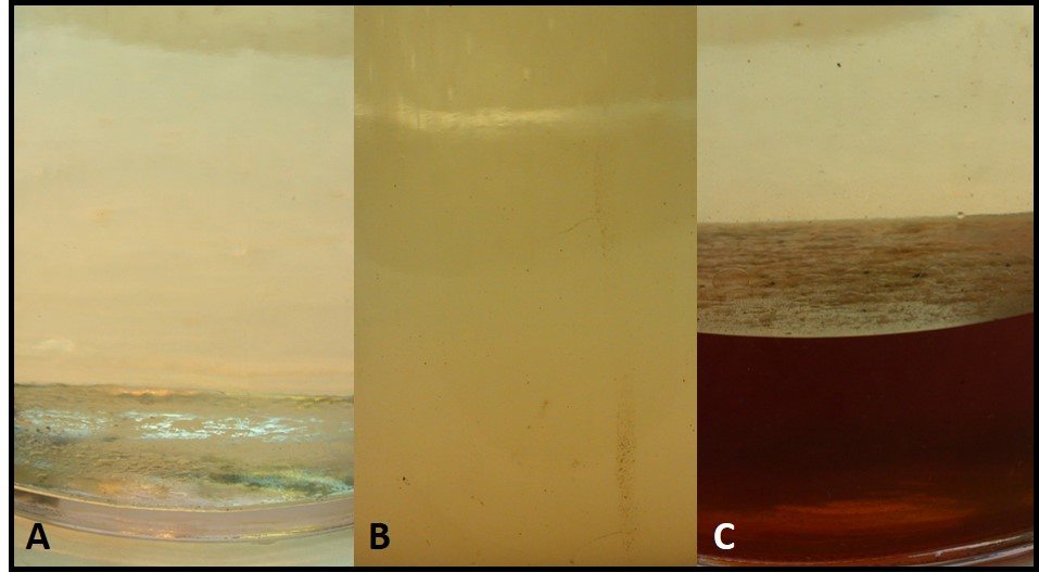
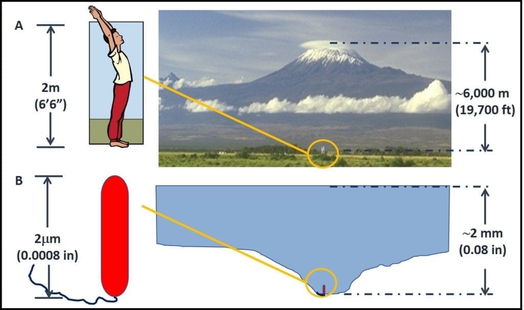
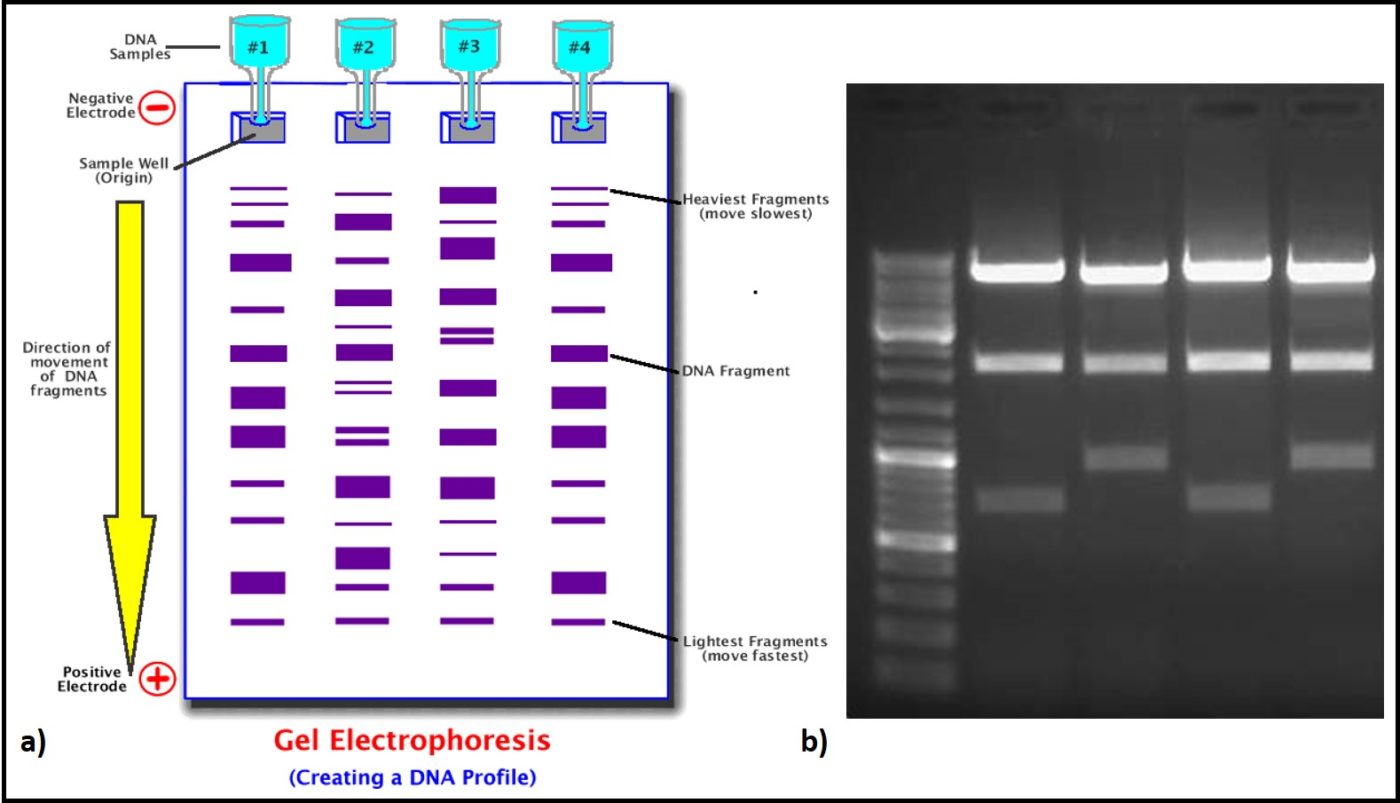
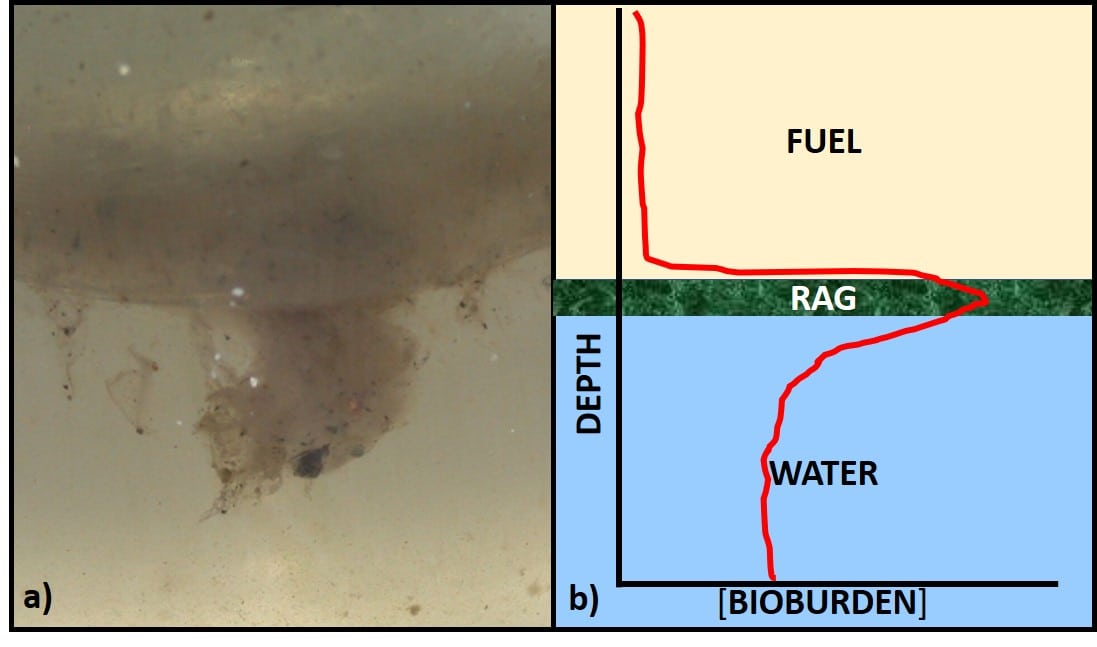
Most often we base fuel treatment decisions on test results from bottoms samples. Growth at the fuel-water interface can be seen either as an invert (water in oil) emulsion (rag-layer), membrane-like layer (pellicle), or both (fig 1a). Profiles of bioburdens in fuel, interface, bottoms-water layers generally show that the greatest bioburden is in the interface layer (fig 1b).

Fig 1. Fuel-water interface. 1a: fuel over water, separated by rag-layer; 1b) schematic profile showing maximum bioburden within rag-layer, minimum in fuel, and intermediate bioburden in bottoms-water.

Biofilms
In Part 15 (November 2017), I wrote about biofilms. Biofilms are complex, slimy residues that can form at the fuel-water interface (as in fig 1a) and on fuel system surfaces, including bottom-sludge and sediment. Among their numerous fascinating properties, biofilms can act like a slime fortress – preventing microbicides from reaching biofilm microbes.

Treatment objective(s)
Based on the previous section, it should now be clear that most commonly, the objective is to disinfect fuel system surfaces. Treated surfaces can include any combination tank walls, pipe surfaces, valves, meters, and pumps. Treated surfaces will not include the tank ullage zone. If fuel is not in direct contact with a surface, neither will the microbicide. I’ll discuss disinfecting ullage surfaces in my next blog post (Part 23). If only tank surfaces need to be disinfected, then static soaking can be sufficient. However, if the objective includes disinfection of other fuel system component surfaces, the treated fuel will have to be recirculated to ensure that they are exposed to the microbicide.

Dosing
Choosing the correct dose
Dosage is the volume of microbicide added per gallon of fuel (recall from Part 21 that I recommend against doing before removing bottoms-water). All microbicides list minimum and maximum dosages on their container labels. The minimum dose is based on laboratory tests that can provide optimistic results. I always recommend using the maximum permissible dose. Maximum dosage is based on the regulatory agency’s toxicological risk assessment of the microbicide’s active ingredient(s).
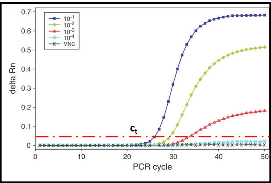
I recommend using the maximum permissible dose because the concentration of microbicide available to kill microbes begins to decrease once the product has been added to the fuel. Collectively, the factors contributing to the disappearance of microbicide active ingredient are called demand. There are chemical, physical, and microbiological demands. Figure 2 illustrates how microbicide concentration can decrease over time. The time axis in fig. 2 can range from hours to months.

Fig 2. Microbicide demand curve.

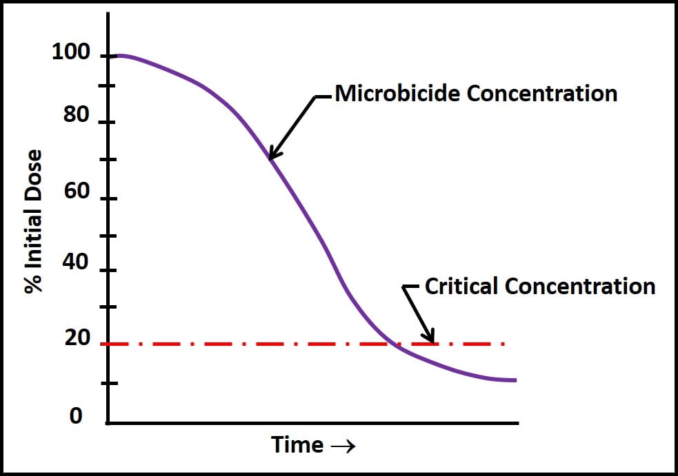
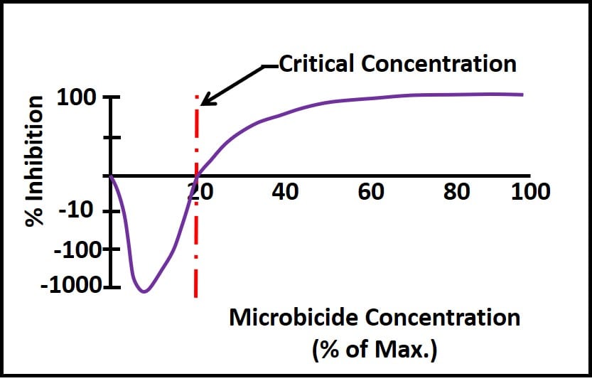
The most common physical demand is dilution. Each time untreated fuel is added to a tank containing treated fuel, it dilutes the microbicide concentration. Figure 3 illustrates what can happen once the microbicide concentration decreases to below its critical concentration – the minimum concentration at which the active ingredient is effective. Note how active ingredients that are quite effective when used as directed can actually stimulate growth once their concentration is less than the critical concentration. In fig. 2, microbial populations exposed to sub-critical microbicide concentrations are more than three orders greater than those in untreated systems. Conversely, at concentrations ≤50 % of the maximum permissible dose, the microbicide is fully effective.

Fig 3. Microbial population response to different microbicide doses (hormesis).

Dosing plan
Although a single dose is often sufficient when treating a lightly contaminated system, it can be insufficient for disinfecting moderately to heavily contaminated systems. The reason is microbicide demand. An effective treatment exposes microbes to adequate concentration of active ingredient for a sufficient period of time (the soak period). The optimal soak period is between 24h and 48h. Except for long-term storage tanks, operators rarely have the luxury of allowing their fuel tanks to stand idle for this long. Depending on the fuel turnover rate, it might be necessary to add microbicide in order to maintain the active ingredient’s effective concentration for at least 24h (this is most commonly an issue at sites that receive more then one fuel delivery per day).

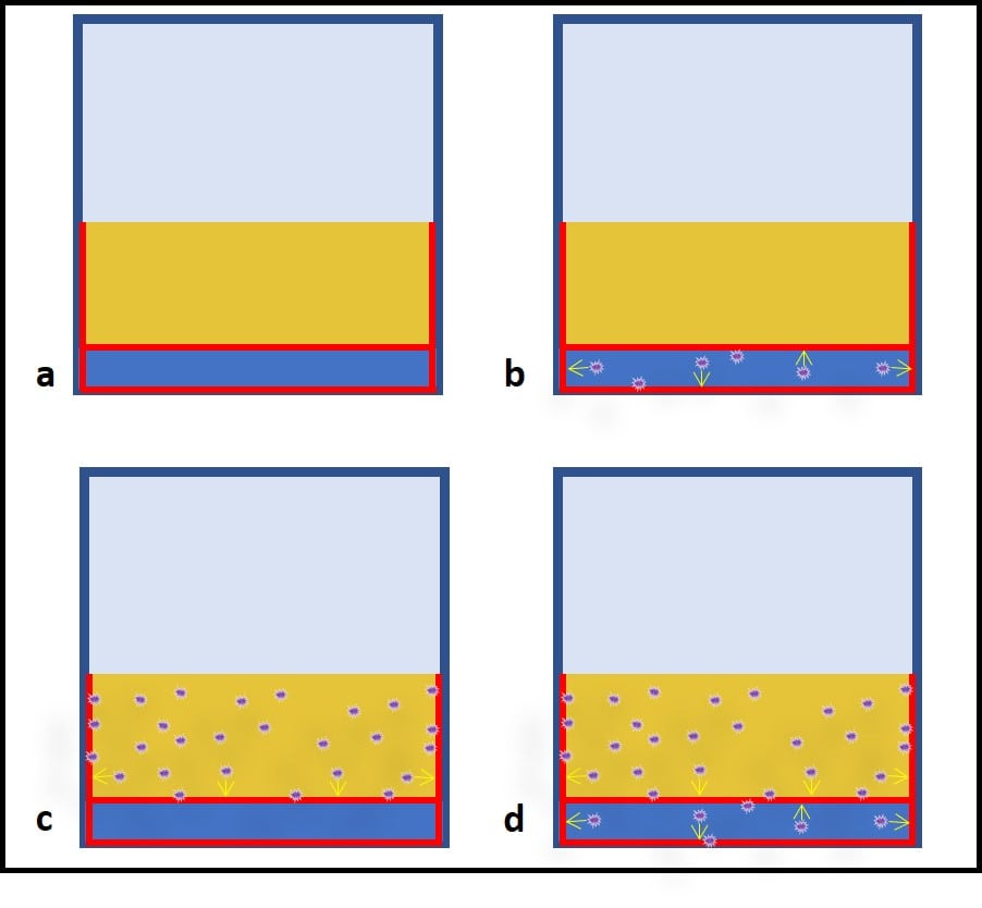
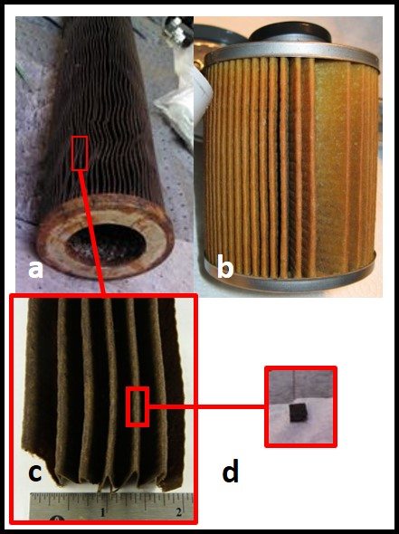
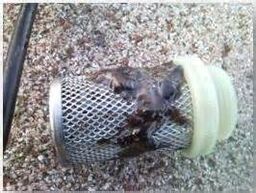
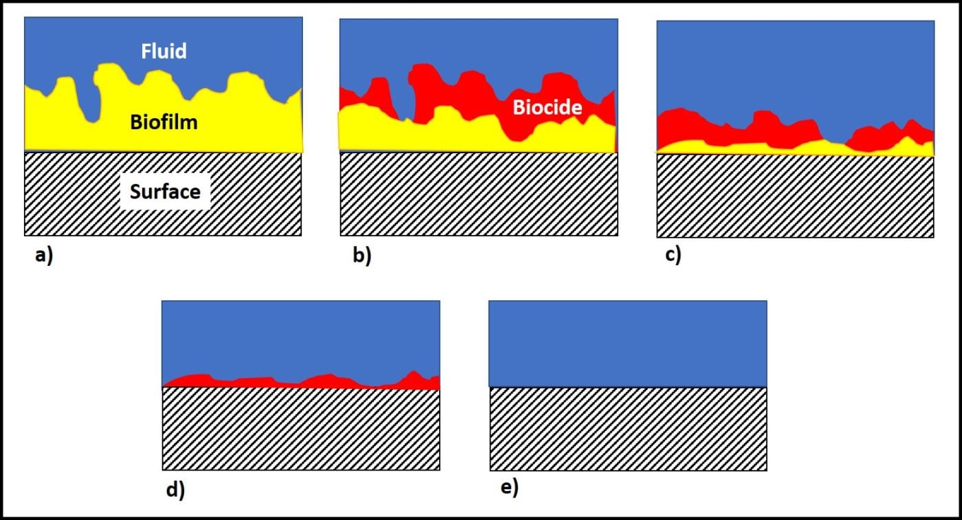
Additionally, active ingredients are used up as they react with microbes. The more heavily contaminated a tank is, the more quickly the available microbicide concentration will decrease. Figure 4 illustrates a point I made above, regarding biofilms. The initial treatment is unlikely to remove the entire biofilm or to kill microbes deep within the biofilm matrix. One or more follow-up treatments might be needed to fully eradicate the biofilm community (fig. 4c, d, and e). Each treatment will cause masses (flocs) of biofilm material to slough away from the surface to which it was originally attached. Some of these flocs will settle to the tank’s bottom. Those that don’t will remain suspended in the fuel and be transported to filters. Rapid filter plugging is a common result of effective biofilm destruction.

Fig 4. Biocide interacting with biofilm – a) biofilm accumulation on a surface; b) first biocide dose penetrates into the biofilm partially, causing some biofilm material to slough off; c) second biocide dose treats most of the remaining biofilm; d) third does disinfects surface; e) after effective treatment, surface is biofilm-free.

When tanks or sufficiently contaminated to cause filter plugging after biocide treatment, polishing, fuel tank cleaning or both should be part of the remedial effort. In part 23, I’ll write about fuel polishing and tank cleaning. In the meantime, if you have questions or comments about today’s post, please contact me at fredp@biodeterioration-control.com.

Disclaimer:
Microbes are ubiquitous. There are extraordinarily few habitats on earth where thriving, microbial communities have not been detected. In practical terms, this means that it is unlikely that operators will ever have a completely sterile fuel system or that they will reduce their fuel system biodeterioration risk to zero. Biodeterioration can still occur in the best maintained fuel systems. However, the risk of it occurring in an inadequately maintained system is much more likely

FUEL & FUEL SYSTEM MICROBIOLOGY PART 21 – PREVENTING MICROBIAL DAMAGE TO FUEL SYSTEMS PART 4; TREATING SYSETMS WITH MICROBICIDES

Fig 1. Microbes in fuel systems and the biocides used to control them – a) fuel (yellow-orange) over bottoms-water (dark blue), with red lines showing where microbes tend to accumulate; b) after treatment with water-soluble biocide (purple stars); c) after treatment with fuel-soluble biocide; d) after treatment with universally-soluble biocide.

Where are the bugs? If you intend to use a biocide to disinfect a fuel system, the first question to ask is: “Where are the bugs?” Figure 1a shows where microbes tend to be most abundant in fuel systems. The red lines symbolize microbe accumulations in the bottoms sludge and sediment, at the fuel-water interface, and on tank walls. Fuel treatment microbicides Microbicides are chemicals that are manufactured and sold for the purpose of killing microbes. They are part of a greater family of chemicals called pesticides or biocides. Formally, microbicides are called antimicrobial pesticides – i.e., they are pesticides that target microbes. I’ll come back to the issue of pesticide registration at the end of the post. For now, I want to split the biocides used for fuel and fuel system treatment into three groups:

1. Water-soluble
2. Fuel-soluble
3. Universally-soluble

Why should I care whether my biocide is water, fuel or universally soluble? Water-soluble biocides Water soluble biocides fall through the product and dissolve into the water-phase (figure 1b). They are not present in the fuel for a long enough period (see Fuel and Fuel System Microbiology Part 22) to kill microbes either in the fuel-phase or on tank walls exposed to fuel. They can effectively kill microbes in bottoms-water, sludge and sediment, but it is reasonable to ask whether this makes good sense. Typically, when water, sludge, and sediment are vacuumed or drained out of tanks, the wastes are shipped to a biological wastewater treatment plant. Biological wastewater treatment depends on microbes to eat organic molecules to reduce the water’s biochemical oxygen demand (percentage of organic matter that microbes can digest in a five-day period), chemical oxygen demand (percentage of organic matter that is chemically oxidizable – convertible to carbon dioxide), and total petroleum hydrocarbons (TPH). I have never understood the logic for killing microbes that can help the waste treatment process, just before shipping those microbes to waste treatment. Therefore, I have never understood the logic of treating fuels or fuel systems with water soluble biocides. Fuel-soluble biocides Fuel-soluble biocides (figure 1c) mirror the performance of their water-soluble cousins. These products effectively kill microbes in the fuel and can be somewhat effective against microbes growing on tank walls in contact with the fuel. They can also attack microbes living at the fuel-water interface. They do not contact microbes living either on tank bottoms or on those portions of the tank wall that are in contact with water rather than fuel. Universally-soluble biocides As their name implies, universally-soluble biocides (figure 1d) can disperse within both the fuel and water phases. Typically, they are fully soluble in fuel and partially soluble in water. Most importantly, they are chemically stable in both phases. As figure 1d illustrates, they can interact with microbes in fuel, in water, at the fuel-water interface, and on all tank surfaces in contact with fuel or water. Consequently, universally-soluble biocides are the most reliable products for disinfecting fuels and fuel systems. Regulations Pesticides are regulated by the U.S. EPA in the USA. Under the U.S. Federal Insecticide, Fungicide and Rodenticide Act (FIFRA – 7 U.S.C. §136 et seq. [1996]), EPA’s Office of Pesticide Programs had direct responsibility for pesticide registration and management. The details of biocide regulations are found in 40 CFR Chapter I, Subchapter E, Parts 152-180. Outside the U.S., the European Union and many individual countries have regulatory agencies responsible for pesticide approval and oversight. The key point here is that microbicides are highly regulated products. Only registered products may be used. Each registered product has one or more approved end-uses (sites). Two US EPA end-uses sites of interest to us are:

• For use in treating fuel-associated water, and
• For use in fuels.

The language can vary among product labels, but the difference between these two general sites is important. The first site applies to water-soluble biocides. The second one refers to fuel-soluble and universally-soluble biocides. If you are considering a microbicide, read the label carefully and make certain that the product has a use in fuels end-use site. There is another fuel-related regulation: 49 CFR Chapter I, Subchapter C, Part 79 Registration of Fuel and Fuel Additives. The regulations under 49 CFR 79 address the use of fuels and fuel additives. Fuels are comprised of molecules built from carbon (C), hydrogen (H), oxygen (O), nitrogen (N), and sulfur (S). This list of elements has the acronym, CHONS. Fuel additives that contain only CHONS are designated as being substantially similar to fuel (subsim). The American Petroleum Institute (API) has created a consortium of companies who produce subsim products. Once a suitable test method has been developed, the members of the consortium will share the cost of engine emission toxicological tests. Each member’s share will be based on the volume of CHONS product they produce. Recognizing the infinitesimally small volume of fuel treatment microbicides, relative to fuels, API charges microbicide manufacturers a minimal fee for consortium membership. The bottom-line here is that fuel treatment microbicides should have two registrations:

1. A pesticide registration, and
2. A fuel additive registration.

None of the water-treatment microbicides that list a variation on the theme of “for use in treating fuel-associated water” are also registered as fuel additives. Most of the products that list “fuel treatment” as an end-use site, carry both registrations. Just to help confuse users, there are several products that have waivers from the U.S. EPA’s Fuel Programs Manager. These waivers are based on the assumption that the microbicides are used to treat fuel systems rather than fuels, and that none of the product remains dispersed or dissolved in fuel. In part 22, I’ll write about how to use universally-soluble fuel treatment microbicides. In the meantime, if you have questions or comments about today’s post, please contact me at fredp@biodeterioration-control.com.

Disclaimer As in my previous two post, I’ll open with a disclaimer. Microbes are ubiquitous. There are extraordinarily few habitats on earth where thriving, microbial communities have not been detected. In practical terms, this means that it is unlikely that operators will ever have a completely sterile fuel system or that they will reduce their fuel system biodeterioration risk to zero. Biodeterioration can still occur in the best maintained fuel systems. However, the risk of it occurring in an inadequately maintained system is much more likely.

FUEL & FUEL SYSTEM MICROBIOLOGY PART 20 – PREVENTING MICROBIAL DAMAGE TO FUEL SYSTEMS PART 2; WATER BITS

Fig 1. From Rime of the Ancient Mariner, Samuel Taylor Coleridge, 1798

Water, water everywhere…

Samuel Coleridge’s infamous mariner paid dearly for having killed an albatross (figure 1). Do fuel quality managers and personnel responsible for fuel system integrity pay dearly for underestimating the ability of small (<1 oz; 30 mL) pools of fuel-associated-water left behind after water has been nominally purged from a fuel tank? A water bit is any small volume of water that remains in a fuel tank after dewatering (my personal, technical definition).
In Part 20, I wrote: “No water means no bugs. Is it as easy as all that?” I also explained why the short answer to the question was: “No.” For emphasis, I’ll again share figure 3 from Part 20 (figure 2, here):

Fig 2. Scale: how 2 mm of water appears to a bacterial cell.

A – a 6’6” tall man standing at the base of Mt. Kilimanjaro; B- a bacterial cell “standing” in a pool of water that is >2 mm deep; the ratios between the height of Mt. Kilimanjaro and the man in A, and between the depth of the pool of water and the bacterial cell in B are the approximately the same.

What can we do about these traces of water?
I confess that I am not a big fan of dispersants. When water dispersants are used routinely as fuel additives, the dispersed water can act as a corrosive agent; damaging engine components. However, when used to complete the job started by draining or vacuuming most of the free-water out of a tank, dispersants can be quite effective.
Figure 3 illustrates how dispersants work. Most dispersants are organic molecules that have a polar (charged; water-soluble) head and a non-polar (non-charged; fuel-soluble) tail. When added to fuel over water (figure 3b), they move towards anywhere where fuel contacts water (figure 3c) and trap tiny (typically <1 µm; 0.0004 in dia) fuel droplets. The fuel “sees” only the dispersant’s non-polar tails, so the droplets disperse uniformly throughout the fuel (figure 3d). The dispersed droplets (micelles) get transported with the fuel and evaporate during combustion in the engine cylinder.

Fig 3. Dispersant action: a) fuel over bottoms-water; b) dispersant added to fuel – inset shows dispersant molecule with polar head and non-polar tail; c) dispersant heads and tails align in water an fuel phases, respectively; d) dispersants form micelles with water droplet trapped in center; typical droplet size is < 1 μm dia.The use of dispersants is controversial. Dispersant manufacturers and marketers focus on dispersant effectiveness in keeping free-water from accumulating in fuel systems. Moreover, under most circumstances, microbes are unlikely to make use of water trapped within dispersant micelles. Conversely, engine manufacturers focus on the potential for dispersed water to corrode and erode injector nozzles; particularly on modern, high-pressure, common-rail diesel engines. Interestingly, there is at least one additive manufacturer that has tried to promote water-emulsion diesel fuels – diesel with a dispersant that enables the fuel to hold as much as 25 % water. As a microbiologist, I was looking forward to investigating microbial contamination problems in systems that handled 25-75 water-in-diesel blends. But that’s another discussion.
In my next blog, I’ll focus on fuel treatment biocides. In the meantime, if you have questions or comments about today’s post, please contact me at fredp@biodeterioration-control.com.

Disclaimer:
Microbes are ubiquitous. There are extraordinarily few habitats on earth where thriving, microbial communities have not been detected. In practical terms, this means that it is unlikely that operators will ever have a completely sterile fuel system or that they will reduce their fuel system biodeterioration risk to zero. Biodeterioration can still occur in the best maintained fuel systems. However, the risk of it occurring in an inadequately maintained system is much more likely.

FUEL & FUEL SYSTEM MICROBIOLOGY PART 19 – PREVENTING MICROBIAL DAMAGE TO FUEL SYSTEMS PART 2; WATER

Disclaimer:

As in my previous post, I’ll open this post with a disclaimer. Microbes are ubiquitous. There are extraordinarily few habitats on earth where thriving, microbial communities have not been detected. In practical terms, this means that it is unlikely that operators will ever have a completely sterile fuel system or that they will reduce their fuel system biodeterioration risk to zero. Biodeterioration can still occur in the best maintained fuel systems. However, the risk of it occurring in an inadequately maintained system is much more likely.

No water means no bugs. Is it as easy as all that?

Best practice for keeping microbes from growing in fuel systems is to keep them dry. You’ll find this guidance in just about every consensus guidance document (for example ASTM D6469) and peer reviewed paper on the subject; including the ones I’ve written. Of course, there is a catch. In today’s post, I’ll write about why keeping fuel systems water-free is much easier said than done.

Water, water everywhere…

Water in fuel systems is typically present in three forms. Dissolved water is made up of individual water molecules and water droplets that are smaller than 1 m diameter (dia; 1 m = 0.00004 in) in fuel. Fuel containing only dissolve water appears to be transparent – no visible haze. The concentration of dissolved water that a fuel product can hold depends on temperature and product chemistry. Water solubility (also called the product’s water tolerance) increases with product temperature. For example, water solubility in E-10 gasoline increases from 0.2 % (by vol.) to 0.5 % as the product temperature increases from 0 C (32 F) to 20 C (68 F). For products typically sold at retail sites, water solubility is greatest in B-5 biodiesel. Water is least soluble in conventional gasoline.

A – Clear and bright gasoline (ASTM D4176 haze rating: 1; B – gasoline with ASTM D4176 haze rating: 6; C – gasoline over bottoms-water; fuel’s ASTM D4176 haze rating: 3.

Once water concentration reaches its saturation limit, individual molecules join together to form dispersed water. Dispersed water droplet diameters range from 1 m dia to  10 m dia. Fuel haze (see ASTM D4176) increases with the number and size of dispersed water droplets. Droplets that are 10 m are heavy enough to settle out of the product and coalesce to form free water. Free-water can accumulate on tank walls, but is most commonly seen as bottoms water. Figure 1 shows three 87 octane gasoline fuel samples: figure 1A has < 0.1 % water (by vol.), figure 1B has an ASTM D4176 haze rating of 6 (i.e., with dispersed water), and figure 1C shows haze rating 3 fuel over free water.

Ethanol-blended gasoline (E-10)

There was a time when competent fuel chemists argued that phase-separation (i.e.: accumulation of bottoms-water) would never happen in E-10 tanks. They believed that because water was more soluble in E-10 than in E-0, there would never be sufficient water accumulation to drive the fuel-water split. The only problem is that they were wrong. Others argued that even if phase-separation did occur, the water-phase would be approximately 60% ethanol. Everyone (except microbes) knows that 60 % ethanol is a good disinfectant. Microbes couldn’t possibly grow in bottoms-water under E-10; except that they do. Most commonly, I do not detect active microbes in E-10 bottoms-water. On occasion, I do. Others have also reported detecting microbes in E-10 bottoms-water. We are not sure what’s going on (i.e., why the bugs are killed by the ethanol), but it is no doubt interesting. Bottom-line: do not assume that underground storage tanks (USTs) containing E-10 do not have bottoms-water or that bottoms-water under E-10 is microbe-free.

Implications

Assume that most UST have some free water. Here’s why:

As explained above, depending on the fuel grade, good-quality quality (i.e., fit-for-use) product can as much as 0.5 % dissolved water.
It is reasonable to assume that in a fuel carrying 0.01 % (i.e., 100 ppm) water, approximately 10 % of that water will separate from solution while product is in a UST. That 10 % of 100 ppm translates to 10 gal per million gal (a retail site that receives a 7,000-gal delivery every two to three days receives approximately 1 million gallons per year).
Based on the previous bullet, approximately 10 gal of water will accumulate, if no other water enters the tank. Figure 2 illustrates this scenario. It shows three-years’ water accumulation in a 10,000 gal (8 ft diameter x 27 ft long underground storage tank; 10 gal = 0.3 in to 0.5 in water).

Figure 2. Underground storage tank (UST); 10,000 gal capacity, with  1 in (30 gal) water.

End and side view of UST that is approximately half filled with product. 1 in of water is approximately 30 gal; barely visible in this schematic. If water does not enter UST by any other means, it can take three years for this volume to accumulate.

End and side view of UST that is approximately half filled with product. 1 in of water  30 gal; barely visible in this schematic. If water does not enter UST by any other means, it can take three years for this volume to accumulate.

Using water-paste on a sounding stick, it should be easy to detect bottoms-water long before 1 in of water has accumulated. In fact, many companies specify that UST should be dewatered whenever 0.5 in or (10 gal to 15 gal) more water is detected. This guidance is based on two key assumptions:

1. USTs rest at the same angle at which they were installed: 1 in per 10 ft grade; with fill-line at low end (figure 3A).
2. UST floors (longitudinal, bottom dead-centerline) are straight (i.e. UST bottoms are flat). In the words of the song from Porgy and Bess: “taint necessarily so.”

There is a problem with these assumptions. USTs are installed on top of backfill. Despite best efforts to fully compact backfill before placing a UST, the tank’s weight – particularly after it has been filled – will cause additional backfill compaction (i.e., settling).

As illustrated in figures 3B and 3C, UST bottoms can settle flat or with the end opposite the fill-line (often the end with the submerged turbine pump – STP) lower than the fill-end. Tanks can also sag (lower in the center than at either end; figure 3D) hog (lower at both ends than in the center; figure 3E), or have numerous peaks and valleys along the longitudinal bottom centerline.

Figure 3. How USTs settle.

A – Typical, planned configuration: UST is lower at fill-end than at turbine end; B- UST is installed to lie flat; C – UST has settled so that turbine end is lower than fill end; D – UST has settled so that center is lower than ends; E – UST has settled so that ends are lower than center. All angles are exaggerated to illustrate settling issues.

Typically, the distance between peaks and valleys are measured in mm (1 mm = 0.04 in), so they are imperceptible to the naked eye. A 1 in per 10 ft incline is impossible to detect without using a bubble level. However, water will flow to low point(s). Long before free-water is detected, a UST is likely to have numerous, small pools of bottoms-water. Each is a great habitat for fuel-system microbes.

Can pools of 1 ounce (30 mL) water be habitats for microbes?

As illustrated in figure 4, to a bacterium a 2 mm deep pool of water (30 mL; 1 oz.) is like an large lake. In figure 4A, a 6 ft 6 in (2 m) tall man is standing at the foot of Mt. Kilimanjaro (19,700 ft – 6,000 m – tall). Figure 4B shows a bacterial cell (0.5 mm dia x 2 m long) “standing” at the bottom of a pool of water that is 2 mm (0.08 in) deep by 6 mm (0.24 in) wide. The relative height of Mt. Kilimanjaro’s peak over the man in figure 4A and the height of the pool of water over the bacterium in figure 4B is the same. In other words, from the perspective of microbes, traces of water that are undetectable to fuel system operators can be like large lakes to microbes; providing mini-habitats for millions of cells.

Figure 4. Scale: how 2 mm of water appears to a bacterial cell.

A – a 6’6” tall man standing at the base of Mt. Kilimanjaro; B- a bacterial cell “standing” in a pool of water that is approximately 2 mm deep; the ratios between the height of Mt. Kilimanjaro and the man in A, and between the depth of the pool of water and the bacterial cell in B are the approximately the same.

Summary:

In summary, water can be present in one or more of three forms in fuel systems:

Dissolved
Dispersed
Free

It is much easier to prescribe keeping tanks water-free than it is to actually eliminate all water.

In my next blog, I’ll focus on options for minimizing water accumulation in fuel systems. In the meantime, if you have questions or comments about today’s post, please contact me at fredp@biodeterioration-control.com

FUEL & FUEL SYSTEM MICROBIOLOGY PART 18 – PREVENTING MICROBIAL DAMAGE TO FUEL SYSTEMS PART 1

Disclaimer:

I’ll open this post with a disclaimer. Microbes are ubiquitous. There are extraordinarily few habitats on earth where thriving, microbial communities have not been detected. In practical terms, this means that it is unlikely that operators will ever have a completely sterile fuel system or that they will reduce their fuel system biodeterioration risk to zero. Biodeterioration can still occur in the best maintained fuel systems. However, the risk of it occurring in an inadequately maintained system is much more likely.

Biodeterioration:

I’ll also take this opportunity to remind readers that biodeterioration (damage caused by organisms) and bioremediation (using microbes or other organisms to degrade or remove toxic or noxious chemicals) are the flip-sides of the biodegradation coin (figure 1).

Figure 1. Just as the two sides of a coin are its obverse (front) and reverse (back) sides, the two sides of biodegradation are bioremediation and biodeterioration.

Microbes degrade fuel quality and fuel system components. In high-turnover retail systems, product deterioration is unlikely. I consider any tank that is refilled at least weekly to be a high-turnover (or high-throughput) system. The time that product spends in the storage tank is too short for degradation to occur. Studies that investigate the rate at which microbes change fuel chemistry, typically show substantial changes after a month or longer. Consequently, fuel in tanks used for emergency generators, or seasonally operated equipment is at greater biodeterioration risk than fuel in retail underground storage tanks (UST), or frequently operated vehicles. That’s all I want to say about fuel biodeterioration for now. I’ll return to the topic in a future blog post.

For now, I’ll focus on fuel system biodeterioration. Most of the damage caused to fuel system components is caused by biofilm communities (see post #16 https://biodeterioration-control.com/2017/11/). Microbes cause damage either directly or indirectly (more on this in a future post). The most obvious indications of biodeterioration are filter plugging and corrosion. Although it’s typically the first indication of a biodeterioration problem, filter plugging is a late symptom. I often compare it to a heart attack; a late – but often first recognized – symptom of coronary disease.

So how do we substantially reduce fuel system biodeterioration risk? Step one is cost-effective condition monitoring (CM). Step two is cost-effective predictive maintenance (PdM; see https://biodeterioration-control.com/microbial-damage-fuel-systems-hard-detect-part-5-predictive-maintenance-pdm/). The former drives the latter. Why do I emphasize cost-effectiveness? As I see it, there is as little justification for investing $10,000 per year to detect problems that might cause $1,000 per year of damage, as there is in refraining from spending $10,000 per year to detect problems that could cost $100,000 per year. I’m not suggesting that any fuel system CM program should cost $10,000 per year. An effective program can cost less than $2,000 per year. My point here is that before setting up a CM/PdM program, stakeholders should invest a bit of time and effort to determine their actual annual biodeterioration-related costs.

Opportunity Cost:

Nearly two decades ago, I first argued that a 10% flow-rate loss at high-traffic, retail sites, can easily translate to more than $100,000 per dispenser per year opportunity cost (Passman, F.J., 1999. “Microbes and Fuel Retailing: The Hidden Costs of Quality.” Nat. Petrol. News 91 [7]: pp: 20-23). My model did not include lost C-store revenues related to customer discontent with their fueling experience. Retailers who have tested my model have invariably been shocked by the huge impact of seemingly minor flow-rate reductions on fuel sales volumes. I’m still trying to understand the psychology behind retailers’ general reluctance to even test my model (for model details, contact me at fredp@biodeterioration-control.com). Bottom line: the return on investment (ROI) for well-designed and executed, CM can easily be >$1,000 return on each $1 invested.

Condition Monitoring:

In Parts 2 through 18 of this series, I’ve written about the details of condition monitoring. I won’t repeat that information here. Instead, I’ll offer a few basic guidelines:

1. Testing hierarchy – CM plans should include two or more tiers. Tests that are easiest and least expensive to perform should be done most frequently (checking UST for bottoms-water accumulation and dispenser flow-rate checks are great examples of Tier 1 tests). Tier 2 tests include bottom-sample visual inspection (optimally, samples should be collected from the fill, automatic tank gauge, and submerged turbine ports). A simple microbiological test (for example ASTM D7687) is indicated whenever the bottom-sample is turbid or when it includes water. When Tier 2 tests indicate that the biodeterioration risk is moderate to high, Tier 3 tests (generally performed by a qualified laboratory) are used to confirm the risk.

2. Test method selection – notwithstanding the examples I mentioned under Testing hierarchy each site owner should develop a CM plan that best meets their needs. You can read my test specific blog posts (or ASTM D6469) for discussions of the benefits and limitations of each test method.

3. Testing frequency – my rule of thumb, after you have determined how often a test parameter is likely to indicate an increased biodeterioration risk, divide that period in three. That gives you the optimal test interval. Testing more often typically translates into greater costs without any real ROI. Testing less frequently increases the risk of having to perform corrective – rather than preventive – maintenance actions.

4. Understanding trends – each of the three previous guidelines depends on a basic understanding of trends. For example, even fuel with an ISO 4406 cleanliness rating of 18/16/13 (see https://www.iso.org/standard/72618.html), will eventually plug dispenser filters. Consequently, dispenser flow-rates will invariably decrease. How many operators know what normal looks like? How many have a control limit? Typically, dispenser filters can process >250,000 gal of fuel before the flow rate will fall below 7 gpm. Replacing fuel filters when the flow-rate is <7 gpm strikes a balance between the opportunity maintenance costs. Knowing whether the flow rate has fallen to <7 gpm after 50,000 gal or 500,000 gal of fuel have been filtered serves to trigger additional sampling and testing. If the amount of fuel filtered before substantial flow reduction occurs is much less than expected, then additional testing is indicated.

Summary:

In summary, microbial contamination control depends on a good CM program that is linked to a good PdM program. A reasonable investment in CM and PdM should be a fraction of the likely cost impact of not having those programs in place. A cost-effective CM program is driven by an understanding of system trends, definition of the methods that will provide the most useful, actionable information; selection of which tests to run; and determination of sampling and testing frequency. In my next blog, I’ll focus on preventive measures. In the meantime, if you have questions or comments about today’s post, please contact me at fredp@biodeterioration-control.com.

FUEL & FUEL SYSTEM MICROBIOLOGY PART 17 –TEST METHODS – GENETIC TESTING

In today’s blog, I’ll cover the lastest family of microbiology methods used for testing fuels & fuel associated water. These methods fall under the category genomics – the study of genes. Warning: genetic testing is more technically complex than the methods I’ve described in recent posts. I’ll do my best to keep the language as simple as possible.

Genetic methods have evolved substantially over the past 30 years. They all depend on the polymerase chain reaction (PCR); first reported in 1983. The common steps of all PCR methods include:

   1) Genetic material (deoxyribonucleic acid – DNA) extraction (fig 1).
   2) Heating to separation of the two strands of DNA’s double helix (fig 2) into two single-strands.
   3) Cooling and using an enzyme – polymerase – to convert each single strand back into double stranded DNA (fig 3).
   4) Repeating steps 2 and 3 until there are millions of copies of each of the DNA originally extracted in step 1.
   5) Using analytical tools to: identify the different types of DNA that were extracted from the original sample in step 1.

Fig 1. Bacterial cell lysing and ejecting its cytoplasm

Fig 2. a) DNA molecule ; b) section of DNA being denatured to two single strands.

Fig 3. Denatured DNA (left) coupled with primer and reacted with DNA polymerase to form two new double helices.

When PCR methods were first developed in the mid-1980s, DNA was extracted from colonies that had developed on nutrient agar plates (see Part 12 and fig 4). Early PCR testing revolutionized microbial taxonomy. Microbes that seemed to be closely related because of their appearance and nutrient preferences turned out to be quite distant genetic relatives. Conversely, some microbes that had historically been classified as being members of different groups, were discovered to be nearly identical genetically. However, PCR could only be used to identify microbes that formed colonies.

Fig 4. Bacterial colonies on nutrient agar.

In the 1990s quantitative-PCR (qPCR) methods were developed. In qPCR, messenger-RNA (mRNA) is extracted and used to synthesize complimentary-DNA (cDNA). The PCR process then continues as described in steps 2 through 5. The RNA used for qPCR is typically tagged with a fluorescent dye. A fluorometer is used to measure the DNA concentration as a function of time during repeated cycles of heating and annealing (steps 2 and 3). As shown in fig 5, the time required for the fluorescence to reach a threshold value, can be used to compute the amount of mRNA that was originally extracted from the sample. This, in turn provides an accurate estimate of the population density (i.e., cells/mL) in the sample.

Fig 5. DNA amplification curves: delta Rn is the amount of fluorescence detected and ct is the threshold delta Rn used to compute the DNA concentration in the original sample. The five curves show that the number of PCR cycles needed to reach ct increases as the original DNA concentration decreases.

Four molecules (nucleotides) make up the genetic code (adenosine – A, cytosine – C, guanine – G, and thiamine – T). Each three-nucleotide sequence is the code for a specific amino acid. Thus, long strings of three-letter messages specify the amino acid sequence of enzymes – the cell’s machinery for carrying out all of life’s processes. The total genome of each type of cell (operational taxonomic unit – OTU) is unique. Because each of the four nucleotides – A, C, G, and T – has a unique electrical charge, each OTU’s DNA has a unique net electrical charge. Using a technique called gel electrophoresis, after amplification (step 5) analysts can separate and isolate each type of DNA that was recovered from the original sample (fig 6). They can then sequence the genes and attempt to match the sample’s DNA against a DNA library. The result is a taxonomic profile of the microbes that were present in the original sample.

Fig 6. DNA profiling using gel electrophoresis: a) schematic illustration of process ; b) photograph of gel.

In earlier posts, I’ve referred to Donald Rumsfeld’s “unknown unknowns.” Although qPCR and, the more recently variation called next generation sequencing – NGS, is a powerful tool for studying microbial communities in fuel systems, it is probably not the last word in microbiology testing. True, qPCR detects many types of microbes that are undetectable by historically used culture methods. However, extracting DNA or RNA from cells is as much art as science. Genetic material that isn’t extracted isn’t detected. Additionally, qPCR testing depends on the use of primers – short sections of mRNA selected to either be universal (i.e., include a section of A, C, G, T basis that are believed to be present in all bacteria) or specific (i.e., include a section of genetic coding that is unique to a microbe of specific interest). Consequently, researchers are on a steep learning curve about how to select primers. As task force within ASTM D02.14 has just restarted work on a qPCR standard test method for fuels and fuel associated water. The last attempt stalled when participants could not agree on a consensus DNA extraction protocol. As the new task force makes progress I provide readers with updates. The goal is to develop a method that non-technical folks will be able to use.

In the meantime, please contact me at fredp@biodeterioration-control.com you’d like to learn more about fuel system microbiology or microbiological contamination control.

Footnotes:

Source: http://www.newswise.com/images/uploads/2013/01/9/lysis_cover.jpg.
Source: http://www-nmr.cabm.rutgers.edu/photogallery/proteins/gif/dna.gif.
Source: https://laboratoryinfo.com/wp-content/uploads/2015/07/Polymerase_chain_reaction.svg_.png.
Source: https://laboratoryinfo.com/wp-content/uploads/2015/07/Polymerase_chain_reaction.svg_.png.
Source: https://www.microbiologyinpictures.com/bacteria-photos/escherichia-coli-photos/e.-coli-staphylococcu-aureus-colonie.jpg.
Source: https://media.nature.com/full/nature-assets/leu/journal/v17/n6/images/2402922f5.jpg.
Source: http://science.halleyhosting.com/sci/ibbio/biotech/pics/electrophoresisnotes.gif.
Source: https://78.media.tumblr.com/tumblr_lwthmyKO441qzcf71o1_500.gif.

FUEL & FUEL SYSTEM MICROBIOLOGY PART 16 –TEST METHODS – LATERAL FLOW DEVICE

Quick review:

In post #12 I provided an overview of microbiological testing.

Next (post #13) I launched my discussion of non-culture tests.

In posts #14 and #16 – post #15 captured my impressions of the fuel microbiology sessions at two conferences – I discussed how ATP testing could be used to measure microbiological contamination in both liquid and solid samples (surface swabs and sections of filter media).

Before moving on from microbiological test methods, I want to cover two more non-culture test methods. The first – ASTM D8070 (Method for Screening of Fuels and Fuel Associated Aqueous Specimens for Microbial Contamination by Lateral Flow Immunoassay; https://www.astm.org/Standards/D8070.htm) – is another test that can easily be run immediately after collecting a fuel, bottoms-water, or mixed sample. The second, quantitative polymerase chain reaction (qPCR) is a laboratory test that is still too complicated for use by field technicians. I’ll discuss qPCR in my next post.

ASTM D8070 is based on a test kit manufactured by Conidia Biosciences Ltd (http://conidia.com/industry/marine-2/detect-diesel-bug/). The lateral flow device (LFD) technology is very similar to that used for pregnancy tests. A few drops of test fluid are dripped into a well at one end of the LFD, the fluid wicks across a filter pad, and the fluid reacts with an antibody cocktail (a mixture of antibodies designed to detect the target microbes). The kit has six LFD assembled as three pairs on a panel (fig 1). The top pair detects bacteria. The middle pair detects fungi, and the third pair detects one particular type of fungus. Within each pair, one LDF detects high antigen concentrations and the other detects low antigen concentrations. For each microbe category the results are negligible, moderate or heavy (fig 2). Each LFD has a control line (always visible) and a test line (visible only if the antigen concentration is below the LFD’s detection limit). If target microbe molecules (antigens) are present in the sample, the test line remains invisible. Thus, figure 2, shows that the sample had heavy bacterial and moderate fungal contamination levels, and insignificant Hormoconis resinae levels. Historically, some fuel microbiologists were convinced that H. resinae was the predominant microbe that contaminated fuels. I suspect that the D8070 kit has retained the H. resinae LFDs for nostalgic, rather than technical reasons.

Fig 1. Unused ASTM D8070 panel showing red, control line in each of the six LFD.

Fig 2. Used ASTM D8070 panel. Top row: heavy bacterial contamination (no visible test line on either LFD); middle row: moderate fungal contamination (visible test line on left LFD, but not on right); bottom row: negligible Hormoconis resinae contamination (test lines visible on both LFD).

In 2015 an ASTM interlaboratory study was run on fuel and bottoms-water samples. The samples were tested by ASTM D7687 (Method for Measurement of Cellular Adenosine Triphosphate in Fuel and Fuel-associated Water with Sample Concentration by Filtration) and D8070. A comparison of the bacterial contamination results from the two methods showed 83 % agreement. Recall from post # 12, that each microbiological test method measures something different. Culture tests use microbes’ ability to reproduce and form visible masses (colonies) on nutrient media. The catalase test measures the concentration of an enzyme that’s present in many different types of oxygen-requiring microbes. ATP testing measures the concentration of a universal energy molecule. The LFD test detects antigens that react (actually: bind with) antibodies selected for their diagnostic usefulness. Consequently, strong agreement between two different test methods provides a means of validating both methods.

No method is without its limitations. D8070 provides attribute scores (three distinct categories) rather than quantitative results. For some users, this might be sufficient. Other users might prefer quantitative results (for example CFU/mL or pg ATP/mL). Inexperienced users might see test lines that are not there (for example, if you look very closely at figure 1, you can see a very faint test line on the unused, top right LFD), or miss lines that are. Still the method is useful for quickly distinguishing between bacterial and fungal contamination. In selected cases, I find it to be a great tier 2 test. If I detect sufficient ATP, I’ll run D8070 to determine whether the ATP is bacterial, fungal, or a combination of both.

If you’d like to learn more about fuel system microbiology, please contact me at fredp@biodeterioration-control.com.

FUEL & FUEL SYSTEM MICROBIOLOGY PART 15 – TEST METHODS – HOW DO WE DETECT BUGS ON SURFACES?

In my August post (https://biodeterioration-control.com/microbial-damage-fuel-systems-hard-detect-part-14-test-methods-still-microbiological-tests/), I discussed using ASTM D7687 to quantify microbial loads (AKA bioburdens) in liquid samples – fuels and fuel associated water. This post will focus on surface samples.

Generally speaking, microbes tend to be most abundant on surfaces. By some estimates, in any given system, for every microbe floating in the bulk fluid, there are 1,000 to 1,000,000 growing on surfaces. These surface microbes are invariably part of biofilm communities. I’ll discuss biofilms in more detail in a future post. For now, it is sufficient to understand that biofilms are slime-encased microbial communities growing on surfaces (fig 1). It is much easier to grab a fluid sample than a surface sample. Consequently, most fuel system samples – even those intended for microbiology testing – are fluids. However, there are a few fuel system surfaces that can be sampled relatively easily.

Fig 1. Scanning electron micrograph of a mature biofilm. Note its structural complexity. Source http://drandreastevens.com/wp-content/uploads/2016/02/Biofilm-Photo.png

Fig 2. Automatic tank gauge, water float showing slime accumulation (right) and swabbed area (left).

Biofilms tend to develop on automatic tank gauge (ATG) water floats (fig 2). The left side of the water float shown in figure 2 has been swabbed. The right side shows the undisturbed deposit. This deposit includes microbes, their slime, and metal fins (i.e. rust). Most often, I use a swab to collect a sample from a premeasured surface area. If the deposit is > 2 mm (1/8 in) thick, I use a spatula to collect the sample.

The second location I routinely check for microbial contamination is the filter. Figure 3a shows a 76 cm (30 in) filter cartridge. It was one of 16 cartridges in a high-capacity filter housing. However, except for its length, the 76 cm cartridge does not look very different from the filter element inside a typical fuel dispenser filter (fig 3b). To test the filter element for microbial contamination, I first inspect the element visually; looking for slime accumulations or discolored zones. For larger filters, I use an alcohol-disinfected forceps and scissors to cut out a section ( 4 cm x 4 cm; fig 3c), and from that cut out a 1 cm x 2 cm piece of filter medium (fig 3d). For dispenser filters, I cut out a 1 cm x 2 cm piece directly. This is my specimen.

If a dispenser has a screen (fig 4), upstream of the filter I collect either a swab or spatula sample just as I would from the ATG water float.

Fig 3. Fuel filter sampling: a) 60 cm filter element from high-capacity housing; b) dispenser filter element; c) section of filter media taken from element shown in fig 3a; d) 1 cm x 2 cm specimen taken from section shown in fig 3c.

Fig 4. Fuel dispenser prefilter screen partially covered with slime.

Once I’ve collected my surface sample I run LuminUltra Technologies, Ltd, Deposit and Surface Analysis (DSA) test (for more information about the DSA method visit https://www.luminultra.com/dsa/; for a video demonstration, visit https://www.youtube.com/watch?v=VEhpbvtej3E). The method provides me with a rapid, quantitative measure of the bioburden on these fuel system surfaces.

Total ATP concentration ([tATP]) <100 pg/cm2 indicates negligible surface contamination. [tATP] between 100 pg/cm2 and 1,000 pg/cm2 indicates moderate contamination (it’s time for maintenance action). [tATP] ≥ 1,000 pg/cm2 signals that prompt corrective action is needed! If you have weighed out samples, the [tATP] per g threshold levels are the same as those for [tATP] per cm2.

If you’d like to learn more about fuel system surface microbiology, please contact me at fredp@biodeterioration-control.com.

FUEL MICROBIOLOGY NEWS FROM RECENT CONFERENCES

In September, I attended two conferences; each of which included a half-day, fuel microbiology session. Although most of the folks presenting fuel microbiology papers were onboard for both conferences, the information overlap was minor. My overall take home lesson is that when it comes to fuel microbiology, we are all still like the five blind men attempting to describe an elephant (if you are not familiar with this ancient, Indian parable, I invite you to look it up).

Although it has been more than 120 years since the first peer-reviewed paper about fuel biodeterioration was published, there is still much we do not understand. The papers presented at the International Biodeterioration and Biodegradation Society (IBBS17) conference during the week of 04 September and the International Conference on the Stability and Handling of Liquid Fuels (ICSHLF15) the following week shed new light on old questions. At the same time, they highlighted the need for more research.
In a nutshell, in my decades of investigating fuel system biodeterioration, I have often detected substantial microbial communities in tanks that showed no evidence of damage. Just as often, I’ve detected considerable damage in systems that seemed to have negligible microbiological contamination. We might just be getting to the point where we can reasonably investigate why some populations cause damage and others don’t. I’ll get to that in a bit.

For those of you who don’t have the patience or inclination to read this entire post, I’ll start with the highlights:
   1. Anaerobic fuel biodeterioration is an important, but often overlooked component of the overall fuel biodeterioration picture.
   2. Sulfur concentration has no impact of fuel biodegradability.
   3. New test methods, still under development, hold tremendous promise to improving our understanding of fuel and fuel system biodeterioration mechanisms.
   4. Fiber-reinforced-polymer biodeterioration is real.

I had the honor of being the keynote speaker, kicking off the IBBS17 session on fuel microbiology. My presentation focused on just how critical sampling is if microbiology data from fuel systems is going to be either relevant or meaningful. During the session, Prof. Joe Suflita (University of Oklahoma) presented the results of studies he and his team have done on microbiologically influenced corrosion (MIC) caused by anaerobic bacteria (anaerobes are microbes that grow only when there is no oxygen present). His two take-home lessons were:
1. Anaerobes growing in seawater-ballasted diesel tanks cause MIC; and
2. The fuel’s sulfur concentration (HSD to ULSD) does not affect, microbial growth, fuel biodeterioration, or MIC risk.

Next, Dr. Oscar Ruiz (Air Force Research Lab – AFRL, Dayton) summarized his recent work on genomic (techniques that profile microbial communities, based on the types of genetic material present and the relative abundance of each unique type of microbe – based on its unique genetic profile – in a sample) and metabolomic (techniques that determine which genes are turned on and which are turned off) testing of fuels and fuel-associated waters. Per my comment earlier in this post, it’s not unusual to detect heavy contamination, but not see evidence of biodeterioration. I suspect that as metabolomic testing becomes more practical to run on lots of samples, we will gain a critical understanding of the triggers that cause some microbial populations to cause damage and other to be benign. As an aside, I’ll note here that understanding these triggers has become a major focus of human and animal disease research. More often than previously understood, we get sick when microbes on which we normally depend turn rogue. The next great leap in microbiology will be to understand what genetic switches are turned on or off. After that, the key will be to learn what triggers these switching actions. I am very excited about the work that Dr. Ruiz is doing at AFRL.

Mr.Graham Hill (ECHA Microbiology, Ltd.) reviewed his Energy Institute sponsored work on the relationship between water and microbial contamination levels in biodiesel blends. Graham and his colleagues looked to the effect of fatty acid methyl esters (FAME) on dissolved, dispersed, and free water. Importantly, they found a critical relationship between dispersed and free water, and bioburdens. Microbial loads did not increase as dissolved water concentration increased. Only once fuel-associated water became biologically available, did bioburden increase. These results weren’t surprising, but it is always great to see hard data that support conventional wisdom.

Prof. Ji-Dong Gu (University of Hong Kong) shared some of the work he had done as a post-doctoral fellow at Harvard, in the early 1990’s. This U.S. Air Force sponsored research is still the most comprehensive study of fiber-reinforced polymer (FRP) biodeterioration that has been published (Prof. Gu has several peer-reviewed papers covering this work; several years ago, the Fiberglass Tank and Pipeline’s attorney demanded that I remove all reference to FRP biodeterioration from the BCA website www.biodeterioration-control.com). Prof. Gu’s research demonstrated that a diverse range of polymers and fibers (including several that had biocides blended into the polymer) were susceptible to biodeterioration. He showed a number of very elegant electron microscope images that illustrated the attack mechanism. He also presented electrical impedance data that demonstrated that FRP lost structural strength as biodeterioration progressed.

Dr. George Dodos (Technical University of Athens) presented data demonstrating that FAME composition affected both the rate and specific nature of biodiesel (B5) biodeterioration. His work built on previous studies that showed similar results. Biodeterioration is more rapid when FAME molecules have more carbon-to-carbon (C=C) double bonds (this is called: degree of unsaturation). Dr. Dodos’ research focused on examining the chemical changes that occurred in different biodiesel blends. Publications of this sort of corroborative research is essential to scientific progress.

Prof. Egemen Aydin (Istanbul University) wrapped up the IBBS17 fuel microbiology session with his paper on the biodeterioration of water-soluble molecules in navy fuels. As many readers know, the refining processes used to produce LSD and ULSD adversely affect fuel lubricity, oxidative stability, and corrosivity. Although they are primarily fuel-soluble, additives used to restore these properties have some water solubility. Consequently, they are nutrients for microbes growing in fuel-associated water. Prof. Aydin’s presentation illustrated how water-soluble fuel molecules can stimulate bioburden development and biodeterioration.

ICSHLF15 followed immediately on the heels of IBBS17. As I noted above, many of the same actors attended and presented papers at both conferences. I’ll only mention the presentations that were unique to the ICSHLF15 fuel microbiology session.
Dr. Giovani Cafi (Conidia Bioscience, Ltd.) presented research being done at Conidia using genetic tools to detect and quantify anaerobic microbes in fuels and fuel associated waters. As I noted, apropos of Prof. Suflita’s IBBS17 presentation, except for sulfate reducing bacteria, historically, anaerobic microbes in fuel systems have been largely overlooked. Dr. Cafi reported that anaerobes are commonly part of the fuel microbiology community. Clearly, more research is needed to better understand what anaerobes are present and how they contribute to both product and system biodeterioration.

Mr. Gareth Williams (EHCA Microbiology, Ltd.) discussed EHCA’s recent investigations in which they compared the results of different fuel microbiology test methods. Not surprisingly, Mr. Williams reported that culture tests do not covary strongly with non-culture tests. As I discussed in my December 2015 blog post (https://biodeterioration-control.com/microbial-damage-fuel-systems-hard-detect-part-3-testing/), any single culture test is unlikely to detect >0.1 % of the different types of microbes present in a fuel or fuel-associated water sample. Put another way, the culture tests typically used for routine condition monitoring are 99 % likely to miss microbes that are present in samples, but won’t grow in the nutrient recipe used to manufacture the culture test kit. Unfortunately, as a manufacturer of culture test kits, ECHA presents methods comparisons as though culture test data represent a gold standard for microbiology testing. Conversely, in my own experience, I have routinely detected heavy microbiological contamination by non-culture methods in samples that appear to be microbiologically clean, based on culture test results. Interestingly, the ECHA data set indicated that ATP data obtained using a method other than ASTM D7687 appeared to have no relationship to other measures of microbial loads.

In addition to the oral presentations there were several noteworthy ICSHLF15 posters that addressed fuel microbiology issues.
Dr. Joan Kelly (Conidia Bioscience, Ltd.) presented the results of a survey that she and her collaborators performed on microbial contamination in U.S. retail site UST. The team collected samples from UST across two states. Not surprisingly (to me), Dr. Kelly’s team detected moderate to high levels of microbial contamination in most of the sampled UST.

Dr. Marlin Vangsness (University of Dayton Research Institute) presented a poster reporting bioburden in bulk storage tanks. Dr. Vangsness reported that most sampled tanks had moderate to heavy microbial contamination. Moreover, he reported that ATP data obtained using ASTM D7463 did not correlate with other microbiological parameters. Having spent 30 years working to separate interferences that had historically made ATP testing unusable for complex, organic chemical rich fluids like fuels and lubricants, I have argued that ASTM D7463 is an unreliable test method. D7463 does not separate water-soluble organic chemicals and salts from microbes in the test specimen. Consequently, ASTM D7463 results are subject to both positive (high values caused by chemical reactions) and negative (low values caused when chemicals in samples capture the light that is generated by the test reaction – see https://biodeterioration-control.com/microbial-damage-fuel-systems-hard-detect-part-14-test-methods-still-microbiological-tests/ – before the light reaches the detector) interferences. Dr. Vangsness’ poster and Mr. Willams’ presentation both corroborate findings that National Research Defense Canada presented at a NATO conference, nearly a decade ago. In contrast to ASTM D7463, ASTM D7687 (see the previous hyperlink) effectively separates interfering chemicals from microbes before extracting ATP.

Speaking of ATP, Ms. Chrysovalanti Tsesmeli, a doctoral candidate at the Technical University of Athens, presented a poster reporting her use of ASTM D7687 and chemical analysis to explore the effects of FAME and hydrogenated vegetable oil (HVO) on marine diesel fuel biodeterioration. Her work showed that HVO-blended fuels were more biostable than FAME-blended fuels.
Last, but not least, Ms. Silvia Bozzi (Chimec S.p.A.) presented a poster that was similar to Dr. Kelley’s. Ms. Bozzi reported on a survey of retail UST in Italy. As in the U.S., the incidence of moderate to high microbial contamination levels in Italy’s retail site UST is considerably greater than generally recognized by site owners and operators.

One of the particularly gratifying aspects of both conferences was the number of young (i.e. under the age of 40) researchers who are investigating fuel microbiology. These young scientists are applying new techniques to ask new questions and to obtain answers that we cannot get using traditional microbiology methods. Moreover, often the young researchers come from non-microbiology disciplines. Because this reflects a multidisciplinary approach to fuel and fuel system biodeterioration it bodes well for the future of fuel microbiology.
Although I didn’t mention any posters or presentations made by Prof. Fatima Bento or her graduate students, I’ll close this blog with a special call out acknowledging the great research being done by this group at Instituto de Ciências Básicas da Saúde, Sao Paulo, Brazil. Few months pass when I don’t have an opportunity to review manuscripts submitted by members of Prof. Bento’s team. They have made many important contributions to our understanding of ULSD and biodiesel biodeterioration. I’d be sorely remiss if I didn’t mention their fine work.

As always, if you’d like to learn more about fuel and fuel system microbiology testing, please contact me at fredp@biodeterioration-control.com.

METAWORKING FLUIDS, 3RD EDITION NOW AVIALABLE!

Thirteen years after Metalworking Fluids, 2nd Ed. was published, the third edition is now available. Metalworking Fluids, 3rd Ed. Jerry Byers, Ed. has just been published (ISBN, Hardbound: 978-1-4987-2222-3; E-book: 978-1-14987-2223-0) and is available from STLE, CRC Press, or Taylor & Francis.

MWF 3rd. Ed. promises to become the new MWF bible. All of its chapters reflect either substantial updates or all new material. I recommend this new volume most strongly to all metalworking industry stakeholders.

Full disclosure, I wrote Chapter 11 – Microbiology of Metalworking Fluids. Many of the other chapters were written by colleagues on STLE’s Metalworking Fluid Education and Training Subcommittee.

Author Archive

FUEL & FUEL SYSTEM MICROBIOLOGY PART 22 – PREVENTING MICROBIAL DAMAGE TO FUEL SYSTEMS PART 5; TREATING SYSETMS WITH MICROBICIDES – DOSING

FUEL & FUEL SYSTEM MICROBIOLOGY PART 21 – PREVENTING MICROBIAL DAMAGE TO FUEL SYSTEMS PART 4; TREATING SYSETMS WITH MICROBICIDES

FUEL & FUEL SYSTEM MICROBIOLOGY PART 20 – PREVENTING MICROBIAL DAMAGE TO FUEL SYSTEMS PART 2; WATER BITS

FUEL & FUEL SYSTEM MICROBIOLOGY PART 19 – PREVENTING MICROBIAL DAMAGE TO FUEL SYSTEMS PART 2; WATER

FUEL & FUEL SYSTEM MICROBIOLOGY PART 18 – PREVENTING MICROBIAL DAMAGE TO FUEL SYSTEMS PART 1

FUEL & FUEL SYSTEM MICROBIOLOGY PART 17 –TEST METHODS – GENETIC TESTING

FUEL & FUEL SYSTEM MICROBIOLOGY PART 16 –TEST METHODS – LATERAL FLOW DEVICE

FUEL & FUEL SYSTEM MICROBIOLOGY PART 15 – TEST METHODS – HOW DO WE DETECT BUGS ON SURFACES?

FUEL MICROBIOLOGY NEWS FROM RECENT CONFERENCES

METAWORKING FLUIDS, 3RD EDITION NOW AVIALABLE!

Search

Posts

Archives

Categories

Meta

MENU

OUR SERVICES

REQUEST INFORMATION